Application of Split Window Technique for Accurate Land Surface Temperature Measurement from GOES-R
This study explores the Split Window Technique for retrieving Land Surface Temperature (LST) using data from the GOES-R Advanced Baseline Imager. The approach focuses on minimizing the sensitivity to emissivity, view angles, and atmospheric conditions. By evaluating ground-based measurements and conducting sensitivity analyses, the authors aim to enhance the accuracy of LST retrievals. Results demonstrate the algorithm's effectiveness in diverse atmospheric profiles and surface types, emphasizing its potential for operational applications in meteorology and environmental monitoring.

Application of Split Window Technique for Accurate Land Surface Temperature Measurement from GOES-R
E N D
Presentation Transcript
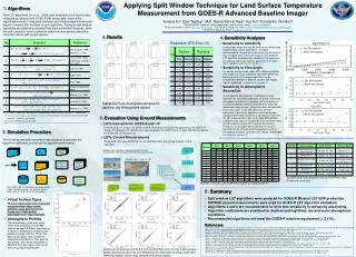
Applying Split Window Technique for Land Surface Temperature Measurement from GOES-R Advanced Baseline Imager Yunyue Yu1, Dan Tarpley2, M.K. Rama Varma Raja3, Hui Xu3, Konstantin Vinnikov4 1NOAA/NESDIS Center for Satellite Applications and Research, email: yunyue.yu@noaa.gov 2Short & Associates, email: Dan.Tarpley@noaa.gov, 3I.M. Systems Group, Inc., email: rama.mundakkara@noaa.gov, hui.xu@noaa.gov 4University of Maryland, email: kostya@atmos.umd.edu 3. Results No Formula# Reference Regression STD Error ( K) 1 Wan & Dozier, 1996; Becker & Li, 1990. No Daytime Nighttime Dry Moist Dry Moist 2 Prata & Platt, 1995; Modified by Caselles et al. 1997. 1 0.35 0.70 0.32 0.92 3 Coll et al. 1997. 2 0.47 0.75 0.47 0.96 4 Vodal, 1991. 3 0.35 0.70 0.33 0.92 4 0.35 0.70 0.32 0.92 5 Price, 1984. 5 0.47 0.72 0.47 0.94 6 Uliveri & Cannizzaro, 1985. 6 0.46 0.75 0.45 0.95 7 0.35 0.70 0.33 0.92 7 Sobrino et al., 1994. 8 0.35 0.70 0.33 0.92 8 Uliveri et al., 1992. 9 0.35 0.65 0.31 0.89 Statistical Plots (histogram samples for daytime, dry Atmosphere cases) 9 Sobrino et al., 1993. # 1) T11 and T12 represent TOA brightness temperatures of ABI channels 14 and 15, respectively; 2) e=(e11+e12)/2andDe=(e11-e12), where e11 and e12 are the spectral emissivities of land surface at ABI channels 14 and 15, respectively; 3) q is the satellite view zenith angle. 5. Evaluation Using Ground Measurements • 4. Sensitivity Analyses • Sensitivity to emissivity • Land surface emissivity may be obtain from surface type classifications or from estimations of satellite measurements. Uncertainty in the emissivity information may introduce error in the LST retrieval. The GOES-R LST algorithm should be less sensitive to the emissivity, yet accuracy improved with the emissivity information. (figure: top/right--sample plots for algorithm 2). • Sensitivity to View Angle • For certain column water vapor (WV), different satellite view angle may result significant absorption difference. Accuracy of the LST retrieval algorithm may be considerably different in different satellite view angles. (figure: middle/right-- sample plots for algorithm2) • Sensitivity to Atmospheric Absorption • In our algorithm development, coefficients of each algorithm are calculated separately for the dry and moist atmospheric conditions. In practice, WV information is usually provided by satellite measurements and/or by radiosonde measurement. Using such data, two possible errors may occur: 1) the WV value may be miss-measured, 2) due to the spatial resolution difference (usually the WV data resolution is significantly lower than the LST measurement), dry-moist mixed atmospheric conditions may occur in a single WV informed area (which usually contains several LST measurement pixels). Therefore, it is possible that coefficients of the LST algorithm for dry atmosphere being applied for moist atmosphere condition, and vise verse (figure: bottom/right-- sample plots for algorithm 2) • LSTs Derived from GOES-8 and -10 • GOES-8 (and -10) Imager has similar thermal infrared channels and view geometry to the GOES-R Imager. The derived LST algorithm has been applied to the GOES-8 and -10 data and then compared to the ground LST estimations. • LSTs Ground Measurements • The ground LSTs were estimated over six SUFRAD sites, every three minutes, for the • year 2001. 2. Simulation Procedure The following simulation procedure was designed to generate the algorithm coefficients and to test the algorithm performance: Site No. Site Location LAT, LONG Surface Type# 1 Pennsylvania State University, PA 40.72N, -77.93W Mixed Forest Algorithm coeffs Atmospheric profiles Input setting 2 Bondeville, IL 40.05N, -88.37W Crop Land 3 Goodwin Creek, MS 34.25N, -89.87W Evergreen Needle Leaf Forest STD Error Of Algorithms 4 Fort Peck, MT 48.31N, -105.10W Grass Land Regression Of LST algorithms MODIS Sensor RSR functions MODTRAN simulation start 5 Boulder, CO 40.13N, -105. 24W Crop Land 6 Desert Rock, NV 36.63N, -116.02 W Open Shrub Land Location and surface types of the six SURFRAD sites. #: UMD land surface type BT Calculation TOA spectral radiances Sensor BTs Algorithm Comparisons end Tool: MODTRAN 4.2, NOAA 88 atmospheric profiles Loops: 60 daytime profiles, 66 nighttime profiles View zenith: 0, 10, 20, 30, 40, 50 ,60 degrees • Virtual Surface Types • 78 virtual surface types were constructed using prescribed unique surface emissivity values determined from Snyder et al.’ (1998) surface classification work. (figure: top/right) • Atmospheric Profiles • 126 atmospheric profiles were used, which were collected from NOAA88 radiosonde and TOVS data, representing a variety of atmospheric conditions and latitude coverage (600 S to 700 N). The figure shows water vapor-surface air temperature distributions of the daytime (60) profiles. Dry (moist) atmosphere is defined if the water vapor is less (more) than 2.0 g. (figure:bottom/right) Scatter plot comparison of GOES-8 LST and SUFRAD LST of all the match-up data. Better statistical results of the LST differences are observed (not shown here) after removing residual noises using seasonal and annual signals. 1. Algorithms Nine LST algorithms (Yu et al., 2008) were analyzed for the land surface temperature retrieval from GOES-R ABI sensor data. Each of the algorithms consists of two parts: the basic split window algorithm and path length correction (the last term in each algorithm). The basic split window algorithms are adapted or adopted from those published literatures, while the path correction term is added for additional atmospheric absorption correction due to path length various. Number of satellite and SURFRAD match-up measurements. • 6. Summary • Split window LST algorithms were analyzed for GOES-R Mission LST EDR production. • SUFRAD ground measurements were used for GOES-R LST algorithm evaluation • Algorithms 2 and 6 are recommended for their less sensitivity to emissivity uncertainty. • Algorithm coefficients are stratified for daytime and nighttime, dry and moist atmospheric conditions. • Recommended algorithms will meet the GOES-R mission requirement (< 2.4 K). • References • Berk, A., G. P. Anderson, P. K. Acharya, J. H. Chetwynd, M. L. Hoke, L. S. Bernstein, E.P. Shettle, M.W. Matthew and S.M. Alder-Golden , MODTRAN4 Version 2 Vehicles Directorate, Hanscom AFB, MA 01731-3010, April 2000. • Wan, Z. and J. Dozier, “A generalized split-window algorithm for retrieving land surface temperature from space”, IEEE Trans. Geosc. Remote Sens., 34, 892- 905, 1996. • Becker, F. and Z.-L. Li, “Toward a local split window method over landsurface”, Int. J. Remote Sensing, vol. 11, no. 3, pp. 369–393, 1990. • Prata, A. J. and C.M.R. Platt, “Land surface temperature measurements from the AVHRR”, proc. of the 5th AVHRR Data users conference, June25-28, Tromso, Norway, EUM P09,443-438, 1991. • Caselles, V., C. Coll and E. Valor, “Land surface temperature determination in the whole Hapex Sahell area from AVHRR data”, Int. J. remote Sens. 18, 5, 1009-1027, 1997. • Coll, C., E. Valor, T. Schmugge, V. Caselles, “A procedure for estimating the land surface emissivity difference in the AVHRR channels 4 and 5”, Remote Sensing Application to the Valencian Area, Spain, 1997. • Vidal, A., “Atmospheric and emissivity correction of land surface temperature measured from satellite using ground measurements or satellite data”, Int. J. Remote Snes., 12, 2449-2460, 1991. • Price, J. C., “Land surface temperature measurements from the split window channels on the NOAA 7 Advanced Very High Resolution Radiometer”, J. Geophys. Res., 89, 7231-7237, 1984. • Ulivieri, C. and G. Cannizzaro, “Land surface temperature retrievals from satellite measurements”, Acta Astronautica, 12, 997–985, 1985. • Sobrino, J. A., Z.L. Li, M.Ph. Stoll, F. Becker, “Improvements in the split-window technique for land surface temperature determination”, IEEE Trans. Geosc. Remote Sens., 32, 2, 243-253, 1994. • Ulivieri, C., M.M. Castronouvo, R. Francioni, A. Cardillo, “A SW algorithm for estimating land surface temperature from satellites”, Adv. Spce res., 14, 3, 59-65, 1992. • Sobrino, J. A., Z.L. Li, M.Ph. Stoll, F. Becker, “Determination of the surface temperature from ATSR data”, Proceedings of 25th International Symposium on Remote Sensing of Environment held in Graz, Austria, on 4th-8th April, 1993 (Ann Arbor, ERIM), pp II-19-II-109, 1993. • Snyder, W. C., Z. Wan, and Y. Z. Feng, “Classification-based emissivity for land surface temperature measurement from space”, Int. J. Remote Sensing, vol. 19, no. 14, pp. 2753-2774, 1998. • Yu, Y, J. Privette, A. Pinheiro, “Evaluation of split window land surface temperature algorithms for generating climate data records”, IEEE Trans. Geosc. Remote Sens., Jan. 2008, in press.