Optimal Scheduling Algorithms for Minimizing Tardiness in Job Processing

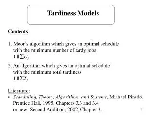
1. Tardiness Models • Contents • 1. Moor’s algorithm which gives an optimal schedule with the minimum number of tardy jobs • 1 || Uj • 2. An algorithm which gives an optimal schedule with the minimum total tardiness 1 || Tj • Literature: • Scheduling, Theory, Algorithms, and Systems, Michael Pinedo, Prentice Hall, 1995, Chapters 3.3 and 3.4 or new: Second Addition, 2002, Chapter 3.

2. Moor’s algorithmfor 1 || Uj Optimal schedule has this form jd1,...,jdk, jt1,...,jtl meet their due dates EDD rule do not meet their due dates Notation J set of jobs already scheduled JC set of jobs still to be scheduled Jd set of jobs already considered for scheduling, but which have been discarded because they will not meet their due date in the optimal schedule

3. Step 1. J =  Jd =  JC = {1,...,n} Step 2. Let j* be such that Add j* to J Delete j* from JC Step 3. If then go to Step 4. else let k* be such that Delete k* from J Add k* to Jd Step 4. If Jd =  STOP else go to Step 2.

4. Example 1 7 1 2 15 7 1 2 3 15 19 7 J =  , Jd =  , JC = {1,...,5} j*=1 J = {1} , Jd =  , JC = {2, 3, 4, 5}, t=7 < 9 = d1 j*=2 J = {1, 2} , Jd =  , JC = {3, 4, 5}, t=15 < 17 = d2 j*=3 J = {1, 2, 3} , Jd =  , JC = {4, 5}, t=19 > 18 = d3 k*=2 J = {1, 3} , Jd = {2}, t=11

5. 1 3 4 5 15 17 23 7 1 3 4 15 17 7 j*=4 J = {1, 3, 4} , Jd = {2}, JC = {5}, t=17 < 19 = d4 j*=5 J = {1, 3, 4, 5} , Jd = {2}, JC = , t=23 > 21 = d5 k*=1 J = {3, 4, 5} , Jd = {2, 1}, t=16 < 21 = d5 optimal schedule 3, 4, 5, 1, 2 Uj = 2

6. k {1, ... ,k-1} any order {k+1, ... ,n} completion timeof job k {k++1, ..., n} any order {1, ... ,k-1, k+1, ..., k+} any order The Total Tardiness 1 || Tjis NP hard Lemma. If pj< pk and dj < dk then there exists an optimal sequencein which job j is scheduled before job k. d1 ...  dn and pk = max(p1, ... , pn) Lemma.There exists an integer , 0 n-k such that there is anoptimal schedule S in which job k is preceded by jobs j k + and followed by jobs j > k +  . k

7. PRINCIPLE OF OPTIMALITY, Bellman 1956. An optimal policy has the property that whatever the initial state and the initial decision are, the remaining decisions must constitute an optimal policy with regard to the state resulting from the first decision. Algorithm Dynamic programming procedure: recursively the optimal solution forsome job set J starting at time t is determined from the optimal solutionsto subproblems defined by job subsets of S*S with start times t*t . J(j, l, k) contains all the jobs in a set {j, j+1, ... , l} with processing time pk V( J(j, l, k) , t) total tardiness of the subset under an optimal sequence if this subset starts at time t

8. Initial conditions: V(, t) = 0 V( { j }, t ) = max (0, t + pj - dj) Recursive conditions: where k' is such that pk' = max ( pj' | j' J(j, l, k) ) Optimal value function is obtained for V( { 1,...,n }, 0)

9. Example k'=3, 0  2 dk' = d3 = 266 V( J(1, 3, 3) , 0) = 0 1, 2C2 = 200 < 266 = d2 T1+ T2 = 0 2, 1C1 = 200 < 260 = d1 T2+ T1 = 0 C3(0) - d3 = 121 + 79 + 147 - 266 = 347 - 266 = 81

10. V( J(4, 5, 3) , 347) 4, 5T4 = 430 - 336 = 94 T5 = 560 - 337 = 229 T4 + T4 = 317 5, 4T5 = 477 - 337 = 140 T4 = 560 - 336 = 224 T5+ T4 = 364 C3(1) - d3 = 347 + 83 - 266 = 430 - 266 = 164 C3(2) - d3 = 430 + 130 - 266 = 560 - 266 = 294 V( J(1, 4, 3) , 0)=0 achieved with the sequence 1, 2, 4 and 2, 1, 4 V( J(5, 5, 3) , 430)=223 V( J(1, 5, 3) , 0)=76 achieved with the sequence 1, 2, 4, 5 and 2, 1, 4, 5 V(  , 560)=0 optimal sequences: 1, 2, 4, 5, 3 and 2, 1, 4, 5, 3

11. Summary • 1 || Uj forward algorithm • 1 ||  wjUj is NP hard • 1 || Tjis NP hard, pseudo-polynomial algorithm based on dynamic programming