Download

1 / 49
520 likes | 727 Vues
Genomics and Personalized Care in Health Systems Lecture 6 Gene Finding (Part 1). Leming Zhou, PhD School of Health and Rehabilitation Sciences Department of Health Information Management. Overview. Basic gene organization The gene annotation problem Methods in gene prediction

E N D
Genomics and Personalized Care in Health SystemsLecture 6 Gene Finding (Part 1) Leming Zhou, PhD School of Health and Rehabilitation Sciences Department of Health Information Management
Overview • Basic gene organization • The gene annotation problem • Methods in gene prediction • Types of information used • Algorithmic approaches • Predictive (ab initio) • Comparative • Combined
Protein Coding Genes • Prokaryotic genes • Generally lack introns • Several highly conserved promoter regions are found around the start sites of transcription and translation • Highly conserved features of prokaryotic genes have made computational gene identification a possibility • One method to detect these genes is to create HMMs based on the gene structures • GeneMark.hmm; Glimmer (Interpolated Markov Models) • Identifies 97-98% of bacterial genes • Eukaryotic genes • More complicated than prokaryotic genes • Major focus of this class
Eukaryotic Gene Organization Model of eukaryotic gene transcription and translation Promoter region Translation start Upstream transcription factor binding sites Gene TATA box DNA coding strand Sp1 Oct1 C/EBP Initiator AAUAAA Transcription cap Exon 1 Exon 2 Intron primary transcript (A)n AG GT 3’ UTR 5’ UTR ATG TGA Splicing mRNA 3’ UTR 5’ UTR Translation protein (peptide)
Genome Annotation • Annotation – Characterizing genomic features using computational and experimental methods • Four levels of genome annotation • Where are genes? • What do they look like? • What do they encode? • What proteins/pathways involved in?
Predicting Genes Computationally • Take the genomic DNA and run it though gene prediction programs to locate genes • Gene prediction programs basing on observed characteristics: • Known exons; Introns; Splice sites; Regulatory sites in known genes • Gene structure varies from one organism to the next • Codon usage pattern vary by species • Functional regions (promoters, splice sites etc) vary by species • Repeat sequences are species-specific • Program trained on one organism is generally not useful for finding genes on another organism
Eukaryotic Gene Prediction • Train a program to recognize sequences that are characteristic of known exons in genomic DNA sequences • Use learned information to predict exons in unknown genomic sequences, and connect exons to produce a gene structure • Patterns used: • intron-exon boundaries • upstream promoter sequences • In eukaryotes, these signals are poorly defined
Locating ORFs • Simplest method of predicting coding regions is to search for open reading frames (ORFs) • ORFs begin with a start (ATG) codon, and ends with one of three stop codons. There are 6 possible reading frames • Locating an open reading frame from a start codon to a stop codon can give a strong suggestion into protein coding regions • Longer ORFs are more likely to predict protein-coding regions than shorter ORFs. • ORF corresponding to a gene may contain regions with stop codons found within intronic regions • Posttranscriptional modification makes gene prediction more difficult
Eukaryotic Gene Annotation • Given an eukaryotic genomic sequence: • Identify the precise location and characteristics of the genes the sequence contains, i.e.: • Exon/intron structure (exon and intron start-end coordinates) • Strand (+ or -) • Start and end sites for translation (ORF) 3’ 5’ CAT 5’ ATG 3’ TAA TTA 10,600 10,135 10,978 11,008 13,410 14,312 18,115 18,423 19,899 20,401 Exon 1 Exon 2 Exon 3 Exon 2 Exon 1 Gene 1 (+ strand) Gene 2 (- strand)
Translation start codon TATA box Gene ATG CpG rich region DNA coding strand AAUAAA Exon 2 Exon 1 primary transcript (A)n AG GT Polyadenylation site Splice signals Types of Information Used Signals • Upstream regulatory signals (TATA boxes) • Translation start codon (ATG) • Translation stop codon (e.g., TAA) • Polyadenylation signal (~AATAAA) • Splice recognition signals (e.g., GT-AG, CT-AC)
Types of Information Used Content • Differential codon usage in coding (biased) versus non-coding sections (uniform distribution) of the gene • Distribution of exon and intron lengths • Distribution of lengths of intergenic regions • Local characteristics of the upstream sequence (CpG islands, C-phosphodiester bond – G, typically 300 – 3000 base pair) 0 5000 10000 0 500 1000 Distribution of exon lengths Distribution of intron lengths
Full-length mRNA ESTs Protein Types of Information Used Similarity • cDNA: single-stranded DNA complementary to an RNA, synthesized from it by reverse transcription • full-length mRNAs • ESTs – Expressed Sequence Tags • Relatively short, 500 bp long on average • May span one or more exons • Large data sets • Protein sequences • Orthologous sequences from related species Genomic DNA
Methods in Gene Finding • Predictive (ab initio) • De novo analysis of genomic sequences(GenScan; HMMer;FGenesH) • Prokaryotes • ORF identification • Eukaryotes • Promoter prediction; PolyA-signal prediction; Splice site, start/stop-codon predictions • Comparative • Comparison of protein and genomic sequences(Procrustes; Genewise) • Comparison of expressed DNA (ESTs, cDNA, mRNA) and genomic sequences (EST_GENOME; SIM4; Spidey) • Cross-species comparisons of orthologous genomic sequences(ROSETTA; CEM; SGP-2) • Combined predictive and comparative (TwinScan; GenomeScan;SLAM) • Similarity Searches (e.g. BLAST, BLAT) • Genome Browsers • RNA evidence (ESTs)
Ab initio Gene Finding • Use information embedded in the genomic sequence exclusively to predict the gene structure. • Primary types of information: signals, content. • Computational models: machine-learning techniques such as Hidden Markov Models (HMMs) or Neural Networks (NNs) • Advantages • Intuitive, natural modeling • Prediction of ‘novel’ genes, i.e., with no a priori known cDNA or protein evidence • Caveats • Not effective in detecting interleaved or overlapping genes, or alternatively spliced forms • Difficulties with gene boundary identification • Danger of over-fitting the model • Potentially large number of false positives
Ab initio Gene Finding • Predictions are based on the observation that gene DNA sequence is not random: • Each species has a characteristic pattern of synonymous codon usage • Every third base tends to be the same • Non-coding ORFs are very short • GenScan, GeneMark (HMMs), Grail II(neural networks) and GeneParser (dynamic programming)
GenScan • Gene finder for human and vertebrate sequences • Probabilistic methods based on known genome structure and composition: number of exons per gene, exon size distribution, hexamer composition, etc • Only protein coding genes predicted • Maize and arabidopsis-optimized versions now available • Accuracy in 50-95% range • http://genes.mit.edu/GENSCAN.html
GenScan • High-level organization • States = basic functional units of a gene • Transitions = order relationships • Emissions (from each state) = sequence ‘generators’ • Probabilities associated with transitions and emissions • Gene structure = the most likely path through the states starting and ending in the intragenic state, given the sequence • Lower-level organization • Complex states = specialized prediction modules for each of the higher-level elements • Exons (marginal, internal, phase-specific) (Markov model, MM) • Introns and intergenic regions (MM) • 5’ and 3’UTRs (MM) • Promoter • Polyadenylation site • Donor and Acceptor splice sites (weight matrices)
Types of Exons • Non-coding exons • 5’ UTR • 3’ UTR • Initial coding exon • AUG to first splice site • Internal exons • 3’ and 5’ splice sites • Terminal exons • 3’ splice to termination codon • Single exon genes
Hidden Markov Model in GenScan Reverse (-) strand F- (5’UTR) F+ (5’UTR) P- (prom) P + (prom) E0 + Einit- I0 + I0 - E0 - Einit+ Esngl+ (single-exon gene) Esngl- (single-exon gene) N (intergenic region) I1 - E1 - E1 + I1 + A- (polyA signal) A+ (polyA signal) I2 - Eterm- E2 + I2 + Eterm+ E2 - T+ (3’UTR) T- (3’UTR) Forward (+) strand Each circle or diamond represents a functional unit (state) of a gene or genomic region. (“Prediction of complete gene structures in human genomic DNA”(1997) Burge and Karlin, JMB 268, p. 86)
Phase • Introns and internal exons in this model are divided according to “phase”, which is closely related to the reading frame. • An intron which falls between codons is considered phase 0; after the first base of a codon, phase 1; after the second base of a codon, phase 2, denoted I0, I1, I2, respectively. • Internal exons are similarly divided according to the phase of the previous intron (which determines the codon position of the first base-pair of the exon, hence the reading frame). • For convenience, donor and acceptor splice sites, translation initiation and termination signals are considered as part of the associated exon in this model
Predicted Genes/Exons by GenScan Gn.Ex Type S .Begin ...End .Len Fr Ph I/Ac Do/T CodRg P.... Tscr.. ----- ---- - ------ ------ ---- -- -- ---- ---- ----- ----- ------ 1.01 Init + 818 881 64 1 1 72 78 42 0.048 1.12 1.02 Intr + 15425 15525 101 0 2 93 98 64 0.305 7.73 1.03 Term + 25193 25309 117 1 0 91 48 107 0.768 5.54 1.04 PlyA + 27155 27160 6 1.05 2.03 PlyA - 28210 28205 6 1.05 2.02 Term - 32130 31928 203 1 2 -35 45 249 0.315 5.85 2.01 Init - 33799 33565 235 1 1 39 80 121 0.272 2.82 2.00 Prom - 40619 40580 40 -3.66
Predicted Gene 3 Gn.Ex Type S .Begin ...End .Len Fr Ph I/Ac Do/T CodRg P.... Tscr.. 3.00 Prom + 62127 62166 40 -2.86 3.01 Init + 65823 68753 2931 2 0 62 90 915 0.532 80.56 3.02 Intr + 68832 69030 199 2 1 90 40 113 0.703 5.62 3.03 Intr + 69433 69521 89 2 2 83 98 -10 0.417 -0.81 3.04 Intr + 77893 78061 169 0 1 14 93 116 0.011 4.22 3.05 Intr + 83851 83977 127 2 1 7 116 109 0.726 5.34 3.06 Intr + 85944 86134 191 0 2 107 58 71 0.996 5.23 3.07 Intr + 89227 89537 311 2 2 96 59 230 0.872 16.93 3.08 Intr + 92770 92857 88 0 1 62 74 46 0.659 0.14 3.09 Intr + 97092 97132 41 1 2 90 107 13 0.258 1.34 3.10 Intr + 103330 103413 84 0 0 85 98 31 0.818 3.82 3.11 Intr + 109348 109402 55 0 1 137 110 4 0.919 6.05 3.12 Intr + 111271 111344 74 2 2 69 98 25 0.773 0.73 3.13 Intr + 112762 112822 61 0 1 46 91 69 0.794 1.31 3.14 Term + 114663 114787 125 1 2 118 42 157 0.999 12.65 3.15 PlyA + 116145 116150 6 1.05
Predicted Genes 4 and 5 Gn.Ex Type S .Begin ...End .Len Fr Ph I/Ac Do/T CodRg P.... Tscr.. 4.07 PlyA - 116290 116285 6 1.05 4.06 Term - 125783 125708 76 1 1 138 50 27 0.166 1.21 4.05 Intr - 132033 131789 245 0 2 125 56 141 0.297 10.90 4.04 Intr - 132404 132270 135 2 0 89 75 150 0.999 14.56 4.03 Intr - 133282 133173 110 2 2 126 81 144 0.999 17.50 4.02 Intr - 134505 134418 88 0 1 81 68 149 0.990 11.74 4.01 Init - 135117 135016 102 0 0 109 60 203 0.998 19.84 4.00 Prom - 136275 136236 40 -7.66 5.00 Prom + 136680 136719 40 -8.96 5.01 Init + 138143 138529 387 1 0 81 105 511 0.986 48.91
Explanation to the Results • Gn.Ex: gene number, exon number (for reference) • Type : • Init = Initial exon (ATG to 5' splice site) • Intr = Internal exon (3' splice site to 5' splice site) • Term = Terminal exon (3' splice site to stop codon) • Sngl = Single-exon gene (ATG to stop) • Prom = Promoter (TATA box / initation site) • PlyA = poly-A signal (consensus: AATAAA) • S : DNA strand (+ = input strand; - = reverse complement strand) • Begin : beginning of exon or signal (numbered on input strand) • End : end point of exon or signal (numbered on input strand) • Len : length of exon or signal (bp) • Fr : reading frame (a forward strand codon ending at x has frame x mod 3) • Ph : net phase of exon (exon length modulo 3) • I/Ac : initiation signal or 3' splice site score (tenth bit units) • Do/T : 5' splice site or termination signal score (tenth bit units) • CodRg: coding region score (tenth bit units) • P : probability of exon (sum over all parses containing exon) • Tscr: exon score (depends on length, I/Ac, Do/T and CodRg scores)
Scores and Probability • The SCORE of a predicted feature (e.g., exon or splice site) is a log-odds measure of the quality of the feature based on local sequence properties. • For example, a predicted 5' splice site with score > 100 is strong; 50-100 is moderate; 0-50 is weak; and below 0 is poor (more than likely not a real donor site). • The PROBABILITY of a predicted exon is the estimated probability under GenScan's model of genomic sequence structure that the exon is correct. • This probability depends in general on global as well as local sequence properties, e.g., it depends on how well the exon fits with neighboring exons. It has been shown that predicted exons with higher probabilities are more likely to be correct than those with lower probabilities.
Predicted Peptide and Coding Sequence • Predicted peptide sequence(s): • Predicted coding sequence(s): • >/tmp/02_24_10.fasta|GENSCAN_predicted_peptide_1|93_aa MLPSSICDVRSASARPRPRLGGGLADNCADLLLGSSMAAPSVELTFFLGILAAGKACGSA RGLRSFWTEAEATAAPEKAFWLKVEVHGVRRTA • >/tmp/02_24_10.fasta|GENSCAN_predicted_CDS_1|282_bp atgctgccttcaagtatctgtgatgtgaggagcgcctctgcccggccgcgaccccgtctgggaggaggtttagctgacaattgcgctgatctcctcttgggctcttccatggcagccccttcggtggagctgacctttttcttgggcatcctggcagcagggaaggcctgcggatcggccagggggctccgatccttttggaccgaggctgaagcaacggctgcaccagagaaggccttctggctgaaggtggaagtgcacggggtccgcagaaccgcctaa
cDNA-Genomic Sequence Comparisons • Use the sequence similarity between the cDNA (EST, mRNA) and the genomic sequences to predict the gene model. • Types of information used: similarity, signals • Algorithmic techniques • sequence alignment algorithms to determine the exons • specialized splice junction detection modules (pattern matching techniques, or statistical modeling) • Caveats • The accuracy of the output depends on the quality of the sequence data • Identifying the true match may be difficult when multiple gene homologs exist • Cannot be used to detect ‘new’ genes
5’ 3’ 1kb 2kb 3kb Genomic DNA 1430 1720 2100 2510 3060 3460 1 291 292 700 701 745 cDNA Exon 2 Exon 1 Exon 3 1 745 cDNA-Genomic Sequence Alignment • Align an expressed DNA (EST, cDNA, mRNA) sequence with a genomic sequence for that gene, allowing for introns and sequencing errors. Seq1 = genomic, 3900 bp Seq2 = cDNA, 750 bp (>gi|10092301) 1430 – 1720 (1-291) 100% -> 2100 – 2510 (292-700) 99% -> 3060 – 3460 (701-745) 99%
Mapping ESTs to Genomic Sequence • Compare genomic DNA and ESTs or cDNAs from same species • Perform similarity searches with ESTs and cDNAs from other organisms • Locates potential exons within genomic sequences • If region matches ESTs with high statistical significance, then it is a gene or pseudogene ESTs ESTs 3’ 5’ Genomic Sequence
BLAST • The quintessential sequence alignment tool • General search tool: several versions exist, which align any types of sequences • Forms the core of more specialized programs, such as cDNA-to-genome sequence alignment tools or syntenic gene prediction programs • Goal: Determine all (statistically) significant similarities between a query sequence and a subject sequence or sequence database. • Method review • Identify exact word matches between the query and subject sequences • Extend all hits in both directions with substitutions, until the score falls X or more below the best score achieved for that hit. This produces a set of HSPs (High-scoring Segment Pairs). • Extend HSPs in both directions allowing for gaps • Report matches scoring above some threshold T, statistically determined
Sim4 • I. Detect basic homology blocks = exon cores • Build a list of gap-free local alignments (HSPs) (‘blast’-like method) • Select a ‘maximal’ subset of HSPs whose order and orientation in the two sequences are preserved • II. Refine the exons: extend or trim the ‘exon cores’ to eliminate ‘gaps’ or overlaps in the cDNA sequence • Overlap: Extend each exon on either side • Gaps: Repeat step I with more relaxed parameters (‘blast’-like method) • III. Refine the introns: splice junction detection • Find the best splice site positions in terms of combined alignment accuracy and conformity to splice signals (GT-AG, CT-AC) (signals) • IV. Generate the alignment • Align exons individually (global dynamic programming) • Connect exon alignments by gaps (introns) to form a global alignment that covers the cDNA sequence
Protein-Genomic Sequence Comparisons • Use the sequence similarity between the protein and the genomic sequence to identify the exon/intron boundaries. • Algorithmic techniques • dynamic programming-based sequence alignment algorithms • profile HMMs to model families of protein domains • specialized pattern recognition modules for splice junction prediction • Caveats • Prediction limited to coding regions (excluding 5’ and 3’ UTRs) • Cannot detect novel genes
AAUAAA Exon 2 Exon 1 human (A)n AG GT P AAUAAA Exon 2 Exon 1 mouse (A)n P AG GT Cross-Species Genomic Sequence Comparison • Use the sequence similarity between genomic sequences from related organisms to infer their common gene model. • Algorithmic techniques • Principle of conservation:exons are conserved, introns vary • Dynamic programming algorithms for sequence comparison • Statistical modeling of the splice junctions and other common transcriptional elements • Caveats • Identification of gene boundaries: similarity may not be restricted to exons alone • Cannot detect genes (or exons) not present in both species
Combining Multiple Methods • Why? • No one method is perfect. No one method can detect everything. • Capture correlations and interdependencies between predictions of individual methods • Reduce the variance / bias of each method • Techniques • AND / OR methods (exons = common regions – AND, all regions - OR) • Majority voting • Statistical modeling, e.g. via Bayesian networks • Combined comparative and predictive models • Otto – results from individual gene predictors are input into GenScan • Ensembl– ab initio predictions are validated by cDNA and protein matches • GenomeScan – integrates cDNA and protein similarity into the predictive HMM model • Human expert curation
Examples Method 1 Method 2 Method 3 Method 4 Genomic axis AND method OR method ‘Majority’ method
Glimmer • Gene finder for bacterial and archaebacterial genomes • Uses an “Interpolated Markov model” approach • Predicts genes with around 98% accuracy when compared with published annotations • No web server but source code is freely available • http://www.cbcb.umd.edu/software/glimmer/
GeneMark • GeneMark is a gene finder for bacterial and archaebacterial sequences • Markov model-based • GeneMark.hmm is designed for eukaryotic gene prediction • Both GeneMark and GeneMark.hmm are available as web servers • GeneMark accuracy in 90-99% range • http://exon.biology.gatech.edu/
Twinscan/N-Scan • Incorporates features of GenScan along with sequence similarity with a second organism • Twinscan is currently available for Mammals, Caenorhabditis (worm), Dicot plants, and Cryptococci. • N-SCAN is available for human and Drosophila (fruitfly). • Web serve and source code are available • http://mblab.wustl.edu/software/twinscan/
Still Many Other Programs • CONTRAST • Exoniphy • Augustus • SGP • Geneid • ACEScan • … • If you are interested in these programs, find the original papers, documentations, and the programs, and try them out
Splice Sites • One pattern that is used by gene finders is the consensus profile found in intron/exon boundaries (splice sites) • Canonical: GT-AG (or CT-AC in the reverse strand) • Alternative: GC, AG • U12 Introns: AT, AC
Accuracy of Genome Annotation • In most genomes functional predictions has been made for majority of genes 54-79%. • The source of errors in annotation: • Overprediction (those hits which are statistically significant in the database search are not checked) • Multidomain protein (found the similarity to only one domain, although the annotation is extended to the whole protein). • The error of the genome annotation can be as big as 25%.
Assessing Gene Prediction Programs • Burset and Guigo (1996) describe methods in order to test gene prediction programs • A set of known coding sequences should be used as data to train the models • A set of known coding sequences is provided to evaluate the success of the model • True Positives (TP): Number of correctly predicted coding regions • False Positives (FP): Number of incorrectly predicted coding regions • True Negatives (TN): Number of correctly predicted non-coding regions • False Negatives (FN): Number of incorrectly predicted non-coding regions • Sensitivity = TP/(TP+FN) • Specificity = TN/(TN+FP)
GenScan Prediction Accuracy http://genes.mit.edu/Accuracy.html
Common Difficulties • Exons in UTR are difficult to annotate UTRs are typically not well conserved. • Smaller genes are not statistically significant so they are thrown out. • Algorithms are trained with sequences from known genes which biases them against genes about which nothing is known.
Gene Finding Strategy • Choose the appropriate type of gene finder • Make sure that you’re using gene finders for microbial (intronless) sequences only to analyze prokaryotic species such as bacteria and archaea • If there is no organism-specific gene finder for your system, at least use one that makes sense • i.e. use a mouse gene finder for rat or rabbit • Use a gene finder created for Arobidopsis for plant genome annotation
Homework 5 • View mouse OLR1 refseq gene (the whole gene) in the UCSC genome browser, click “DNA” to obtain the genomic sequence in this gene locus (adding 1000 bps before the start of the gene locus and the 1000 bps after the end of the gene locus) [10 points] • Use GenScan to predict gene exon-intron structure using the sequence obtained in the first step (include the graphical output, the predicted gene structure, and the predicted gene sequences in your homework). [20 points] • Compare the obtained gene prediction and the annotation given in NCBI genbank record (evaluate each exon), find out whether they have the same number of exons and same length of exons [40 points] • Go through the exercise in the handout (a softcopy of the handout and the corresponding sequences can be found on the courseweb), follow the instructions precisely, save the produced web pages, and answer all the questions (some of them might be difficult but try your best to provide reasonable answers). Put all the saved web pages and your answers to the questions into one zip file. [30 points]