Download
1 / 69
710 likes | 844 Vues
This lecture explores gene prediction within computational genomics, focusing on techniques for annotating genomic sequences. Key topics include identifying genes, exon boundaries, and regulatory elements using computational methods that enhance experimental validation. We discuss prokaryotic gene structures, promoter characteristics, and the significance of the Codon Adaptation Index. Additionally, the lecture emphasizes the importance of probabilistic modeling in gene prediction, illustrated through examples like the Genscan algorithm. Understanding these concepts is critical for advancing genomic research and biological insights.

E N D
Gene prediction and HMMComputational Genomics 2005/6Lecture 9b Slides taken (and rapidly mixed) from William Stafford Noble, Larry Hunter, and Eyal Pribman. Partially modified by Benny Chor.
Annotation of Genomic Sequence • Given the sequence of an organism’s genome, we would like to be able to identify: • Genes • Exon boundaries & splice sites • Beginning and end of translation • Alternative splicings • Regulatory elements (e.g. promoters) • The only certain way to do this is experimentally, but it is time consuming and expensive. Computational methods can achieve reasonable accuracy quickly, and help direct experimental approaches. primary goals secondarygoals
Prokaryotic Gene Structure Promoter CDS Terminator Genomic DNA transcription mRNA • Most bacterial promoters contain the Shine-Delgarno signal, at about -10 that has the consensus sequence: 5'-TATAAT-3'. • The terminator: a signal at the end of the coding sequence that terminates the transcription of RNA • The coding sequence is composed of nucleotide triplets. Each triplet codes for an amino acid. The AAs are the building blocks of proteins.
~ 1-100 Mbp ~ 1-1000 kbp 5’ 3’ 3’ 5’ 5’ 3’ … … … … 3’ 5’ promoter (~103 bp) Polyadenylation site enhancers (~101-102 bp) other regulatory sequences (~ 101-102 bp) Pieces of a (Eukaryotic) Gene(on the genome) exons (cds&utr) / introns (~ 102-103 bp) (~ 102-105 bp)
Most of our knowledge is biased towards protein-coding characteristics ORF (Open Reading Frame): a sequence defined by in-frame AUG and stop codon, which in turn defines a putative amino acid sequence. Codon Usage: most frequently measured by CAI (Codon Adaptation Index) Other phenomena Nucleotide frequencies and correlations: value and structure Functional sites: splice sites, promoters, UTRs, polyadenylation sites What is it about genes that we can measure (and model)?
A simple measure: ORF length Comparison of Annotation and Spurious ORFs in S. cerevisiae Basrai MA, Hieter P, and Boeke J Genome Research 1997 7:768-771
Codon Adaptation Index (CAI) • Parameters are empirically determined by examining a “large” set of example genes • This is not perfect • Genes sometimes have unusual codons for a reason • The predictive power is dependent on length of sequence
General Things to Remember about (Protein-coding) Gene Prediction Software • It is, in general, organism-specific • It works best on genes that are reasonably similar to something seen previously • It finds protein coding regions far better than non-coding regions • In the absence of external (direct) information, alternative forms will not be identified • It is imperfect! (It’s biology, after all…)
Simple HMM : Prokaryotes xm(i) = probability of being in state m at position i; H(m,yi) = probability of emitting character yi in state m; Fmk = probability of transition from state k to m.
Outline: Rest of Lecture • Eukaryotic gene structure • Modeling gene structure • Using the model to make predictions • Improving the model topology • Modeling fixed-length signals
A eukaryotic gene • This is the human p53 tumor suppressor gene on chromosome 17. • Genscan is one of the most popular gene prediction algorithms.
A eukaryotic gene Introns Final exon Initial exon 3’ untranslated region Internal exons This particular gene lies on the reverse strand.
An Intron revcomp(CT)=AG revcomp(AC)=GT GT: signals start of intron AG: signals end of intron 3’ splice site 5’ splice site
Signals vs contents • In gene finding, a small pattern within the genomic DNA is referred to as a signal, whereas a region of genomic DNA is a content. • Examples of signals: splice sites, starts and ends of transcription or translation, branch points, transcription factor binding sites • Examples of contents: exons, introns, UTRs, promoter regions
Prior knowledge • We want to build a probabilistic model of a gene that incorporates our prior knowledge. • E.g., the translated region must have a length that is a multiple of 3.
Prior knowledge • The translated region must have a length that is a multiple of 3. • Some codons are more common than others. • Exons are usually shorter than introns. • The translated region begins with a start signal and ends with a stop codon. • 5’ splice sites (exon to intron) are usually GT; • 3’ splice sites (intron to exon) are usually AG. • The distribution of nucleotides and dinucleotides is usually different in introns and exons.
A simple gene model Intergenic Intergenic Intergenic Gene Transcription start Transcription stop Start End Intergenic
A probabilistic gene model Pr(TACAGTAGATATGA) = 0.0001 Pr(AACAGT) = 0.001 Pr(AACAGTAC) = 0.002 … Intergenic Intergenic 0.25 Intergenic Gene 0.67 Transcription start 1.00 Transcription stop 0.75 Start End 0.33 Intergenic Every box stores transition probabilities for outgoing arrows. Every arrow stores emission probabilities for emitted nucleotides.
Parse S = ACTGACTACTACGACTACGATCTACTACGGGCGCGACCTATGCG P = IIIIIIIIIIIIIIIIIIIIIIIIIIIIIIIIIIIIIIIGGGGG TATGTTTTGAACTGACTATGCGATCTACGACTCGACTAGCTAC GGGGGGGGGGIIIIIIIIIIIIIIIIIIIIIIIIIIIIIIIII • For a given sequence, a parse is an assignment of gene structure to that sequence. • In a parse, every base is labeled, corresponding to the content it (is predicted to) belongs to. • In our simple model, the parse contains only “I” (intergenic) and “G” (gene). • A more complete model would contain, e.g., “-” for intergenic, “E” for exon and “I” for intron.
The probability of a parse Pr(ATGCGTATGTTTTGA) = 0.00000000142 Pr(ACTGACTACTACGACTACGATCTACTACGGGCGCGACCT) = 0.0000543 Pr(ACTGACTATGCGATCTACGACTCGACTAGCTAC) = 0.0000789 Intergenic Intergenic 0.25 Intergenic Gene 0.67 Transcription start 1.00 Transcription stop 0.75 Start End 0.33 Intergenic S = ACTGACTACTACGACTACGATCTACTACGGGCGCGACCTATGCGTATGTTTTGAACTGACTATGCGATCTACGACTCGACTAGCTAC P = IIIIIIIIIIIIIIIIIIIIIIIIIIIIIIIIIIIIIIIGGGGGGGGGGGGGGGIIIIIIIIIIIIIIIIIIIIIIIIIIIIIIIII Pr(parse P| sequence S, model M) = 0.67 0.0000543 1.00 0.00000000142 0.75 x 0.0000789 = 3.057 10-18
Finding the best parse • For a given sequence S, the model M assigns a probability Pr(P|S,M) to every parse P. • We want to find the parse P* that receives the highest probability.
Beyond Simplest Model • Improving the gene model topology • Fixed-length signals • PSSMs • Dependencies between positions • Variable-length contents • Using HMMs • Semi-Markov models • Parsing algorithms • Viterbi • Posterior decoding • Including other types of data • Expressed sequence tags • Orthology
Improved model topology Intergenic 2 • Draw a model that includes introns Intergenic 4 Intergenic 1 Gene Transcription start Transcription stop Start End Intergenic 3
Improved model topology Start Transcription start 5’ splice site 3’ splice site Transcription stop End
Improved model topology Start Transcription start 5’ splice site 3’ splice site 4 intergenics 1 intron 4 exons Transcription stop End
Improved model topology Start Transcription start Initial exon Single exon Internal exon 5’ splice site 3’ splice site Intron Final exon Transcription stop End
Modeling the 5’ splice site • Most introns begin with the letters “GT.” • We can add this signal to the model. 5’ splice site 3’ splice site Intron GT
Modeling the 5’ splice site • Most introns begin with the letters “GT.” • We can add this signal to the model. • Indeed, we can model each nucleotide with its own arrow. 5’ splice site 3’ splice site Intron G T Pr(A)=0 Pr(C)=0 Pr(G)=1 Pr(T)=0 Pr(A)=0 Pr(C)=0 Pr(G)=0 Pr(T)=1
Modeling the 5’ splice site • Like most biological phenomenon, the splice site signal admits exceptions. • The resulting model of the 5’ splice site is a length-2 PSSM. 5’ splice site 3’ splice site Intron G T Pr(A)=0.01 Pr(C)=0.01 Pr(G)=0.97 Pr(T)=0.01 Pr(A)=0.01 Pr(C)=0.01 Pr(G)=0.01 Pr(T)=0.97
Real splice sites • Real splice sites show some conservation at positions beyond the first two. • We can add additional arrows to model these states. weblogo.berkeley.edu
Modeling the 5’ splice site 5’ splice site 3’ splice site Intron
Adding signals Start Transcription start Initial exon Single exon Internal exon 5’ splice site 3’ splice site Intron Final exon Transcription stop Red ellipses correspond to signal models like this: End
Positional Independence Pr(“ACTT”|M) = Pr(“A” at position 1 and “C” at position 2 and “T” at position 3 and “T” at position 4|M) = Pr(“A” at position 1|M) Pr(“C” at position 2|M) Pr(“T” at position 3|M) Pr(“T” at position 4|M) • In general, probabilities of independent events get multiplied. • A PSSM assumes independence among nucleotides at different positions.
In this data, every time a “G” appears in position 1, an “A” appears in position 3. Conversely, an “A” in position 1 always occurs with a “T” in position 3. ACTG ACTT GCAC ACTT ACTA GCAT ACTA ACTT Positional dependence
nth-order PSSM • Normally, PSSM entry (i,j) gives the score for observing the ith letter in position j. • In an nth-order PSSM, each score is conditioned on the preceding letters in the sequence. • The entries A|A, C|A, G|A and T|A should sum to 1. 2nd-order PSSM
nth-order PSSM • Normally, PSSM entry (i,j) gives the score for observing the ith letter in position j. • In an nth-order PSSM, each score is conditioned on the preceding letters in the sequence. • How many rows are in a 3rd-order PSSM for nucleotides? nth-order? The probability of observing an “A” in position 3, given that we already observed a “C” in position 2. 2nd-order PSSM
Conditional probability GCGCAGCCGGCGCCGCCGGCGCCTCCGGGGCGGGCGAGGCAGCCTCATCCTGCG • What is the probability of observing an “A” at position 2, given that we observed a “C” at the previous position?
Conditional probability GCGCAGCCGGCGCCGCCGGCGCCTCCGGGGCGGGCGAGGCAGCCTCATCCTGCG • What is the probability of observing an “A” at position 2, given that we observed a “C” at the previous position? • Answer: total number of CA’s divided by total number of C’s in position 1. • 3/11 = 27% • Probability of observing CA = 3/18 = 17%.
Conditional probability GCGCAGCCGGCGCCGCCGGCGCCTCCGGGGCGGGCGAGGCAGCCTCATCCTGCG • The conditional probability Pr(x|y) = Number of occurrences of y:x Number of occurrences of y:* where * is any letter.
Conditional probability GCGCAGCCGGCGCCGCCGGCGCCTCCGGGGCGGGCGAGGCAGCCTCATCCTGCG • What is the probability of observing a “G” at position 3, given that we observed a “C” at the previous position?
Conditional probability GCGCAGCCGGCGCCGCCGGCGCCTCCGGGGCGGGCGAGGCAGCCTCATCCTGCG • What is the probability of observing a “G” at position 3, given that we observed a “C” at the previous position? • Answer: 9/12 = 75%.
Modeling signals Start Transcription start Initial exon Single exon Internal exon 5’ splice site 3’ splice site Intron Final exon Transcription stop End Red ellipses may correspond to nth-order PSSMs.
Modeling variable-length regions Exon length
Modeling variable-length regions • The easy way, using standard HMMs. • And why that’s not so great. How are variable-length insertions modeled in protein HMMs?
The HMM solution Fixed-length signals 5’ splice site 3’ splice site Intron Variable-length content 5’ splice site 3’ splice site Intron
Codons start translation end translation Single exon 2 1 0 1 2 0 start translation end translation Single exon
The complete model Start Transcription start Initial exon Single exon Internal exon 5’ splice site 3’ splice site Intron Final exon Transcription stop End Red ellipses correspond to nth-order PSSMs. Every arrow contains an invisible box with a self-loop.
A small problem 0.9 • Say that each blue arrow emits one letter. • What is the probability that the intron will be exactly 2 letters long? • 3 letters long? • 4 letters long? 0.1 5’ splice site 3’ splice site Intron
A small problem 0.9 • Say that each blue arrow emits one letter. • What is the probability that the intron will be exactly 2 letters long? 10% • 3 letters long? 9% • 4 letters long? 8.1% 0.1 5’ splice site 3’ splice site Intron