Lecture 14 Secondary Structure Prediction

1. C E N T E R F O R I N T E G R A T I V E B I O I N F O R M A T I C S V U Lecture 14Secondary Structure Prediction Bioinformatics Center IBIVU

2. Protein structure

3. Linus Pauling (1951) • Atomic Coordinates and Structure Factors for Two Helical Configurations of Polypeptide Chains • Alpha-helix

4. James Watson & Francis Crick (1953) • Molecular structure of nucleic acids

5. James Watson & Francis Crick (1953) • Molecular structure of nucleic acids

6. The Building Blocks (proteins) • Proteins consist of chains of amino acids • Bound together through the peptide bond • Special folding of the chain yields structure • Structure determines the function

7. Chains of amino acids

8. Three-dimensional Structures • Four levels of protein architecture

9. Amino acids classes • Hydrophobic aminoacids Alanine AlaA Valine ValVPhenylalanine PheF Isoleucine IleILeucine LeuL Proline ProPMethionine MetM • Charged aminoacids Aspartate (-) AspD Glutamate (-) GluE Lysine (+) LysK Arginine (+) ArgR • Polar aminoacids Serine SerS Threonine ThrTTyrosine TyrY Cysteine CysCAsparagine AsnN Glutamine GlnQ Histidine HisH Tryptophane Trp W • Glycine (sidechain is only a hydrogen) Glycine GlyG

10. Disulphide bridges • Two cysteines can form disulphide bridges • Anchoring of secondary structure elements

11. Ramachandran plot • Only certain combinations of values of phi (f)and psi (y)angles are observed psi psi phi omega phi

12. Motifs of protein structure • Global structural characteristics: • Outside hydrophylic, inside hydrophobic (unless…) • Often globular form (unless…) Artymiuk et al, Structure of Hen Egg White Lysozyme (1981)

13. Secondary structure elements Alpha-helix Beta-strand

14. Renderings of proteins • Irving Geis:

15. Renderings of proteins • Jane Richardson (1981):

16. Alpha helix • Hydrogen bond: from N-H at position n, to C=O at position n-4 (‘n-n+4’)

17. Other helices • Alternative helices are also possible • 310-helix: hydrogen bond from N-H at position n, to C=O at position n-3 • Bigger chance of bad contacts • a-helix: hydrogen bond from N-H at position n, to C=O at position n-4 • p-helix: hydrogen bond from N-H at position n, to C=O at position n-5 • structure more open: no contacts • Hollow in the middle too small for e.g. water • At the edge of the Ramachandran plot

18. Helices • Backbone hydrogenbridges form the structure • Directed through hydrophobic center of protein • Sidechains point outwards • Possibly: one side hydrophobic, one side hydrophylic

19. Globin fold • Common theme • 8 helices (ABCDEFGH), short loops • Still much variation (16 – 99 % similarity) • Helix length • Exact position • Shift through the ridges

20. Beta-strands form beta-sheets • Beta-strands next to each other form hydrogen bridges Sidechains alternating (up, down)

21. Parallel or Antiparallel sheets Anti-parallel Parallel • Usually only parallel or anti-parallel • Occasionally mixed

22. Beta structures • barrels • up-and-down barrels • greek key barrels • jelly roll barrels • propeller like structure • beta helix

23. Greek key barrels • Greek key motif occurs also in barrels • two greek keys (g crystallin) • combination greek key / up-and-down

24. Turns and motifs • Secondary structure elements are connected by loops • Very short loops between twee b-strands: turn • Different secundary structure elementen often appear together: motifs • Helix-turn-helix • Calcium binding motif • Hairpin • Greek key motif • b-a-b-motif

25. Helix-turn-helix motif • Helix-turn-helix important for DNA recognition by proteins • EF-hand: calcium binding motif

26. Hairpin / Greek key motif • Different possible hairpins : type I/II • Greek key:anti-parallel beta-sheets

27. b-a-b motif • Most common way to obtain parallel b-sheets • Usually the motif is ‘right-handed’

28. Domains formed by motifs • Within protein different domains can be identified • For example: • ligand binding domain • DNA binding domain • Catalytic domain • Domains are built from motifs of secundary structure elements • Domains often are a functional unit of proteins

29. Protein structure summary • Amino acids form polypeptide chains • Chains fold into three-dimensional structure • Specific backbone angles are permitted or not:Ramachandran plot • Secundary structure elements: a-helix, b-sheet • Common structural motifs:Helix-turn-helix, Calcium binding motif, Hairpin, Greek key motif, b-a-b-motif • Combination of elements and motifs: tertiary structure • Many protein structures available: Protein Data Bank (PDB)

30. Now we go into predicting Secondary Structure Elements

31. Protein primary structure 20 amino acid types A generic residue Peptide bond SARS Protein From Staphylococcus Aureus 1MKYNNHDKIR DFIIIEAYMF RFKKKVKPEV 31 DMTIKEFILL TYLFHQQENTLPFKKIVSDL 61 CYKQSDLVQH IKVLVKHSYI SKVRSKIDER 91 NTYISISEEQ REKIAERVTL FDQIIKQFNL 121 ADQSESQMIP KDSKEFLNLM MYTMYFKNII 151 KKHLTLSFVE FTILAIITSQ NKNIVLLKDL 181 IETIHHKYPQ TVRALNNLKKQGYLIKERST 211 EDERKILIHM DDAQQDHAEQ LLAQVNQLLA 241 DKDHLHLVFE

32. Protein secondary structure Alpha-helix Beta strands/sheet SARS Protein From Staphylococcus Aureus 1 MKYNNHDKIR DFIIIEAYMF RFKKKVKPEV DMTIKEFILL TYLFHQQENT SHHH HHHHHHHHHH HHHHHHTTT SS HHHHHHH HHHHS S SE 51 LPFKKIVSDL CYKQSDLVQH IKVLVKHSYI SKVRSKIDER NTYISISEEQ EEHHHHHHHS SS GGGTHHH HHHHHHTTS EEEE SSSTT EEEE HHH 101 REKIAERVTL FDQIIKQFNL ADQSESQMIP KDSKEFLNLM MYTMYFKNII HHHHHHHHHH HHHHHHHHHH HTT SS S SHHHHHHHH HHHHHHHHHH 151 KKHLTLSFVE FTILAIITSQ NKNIVLLKDL IETIHHKYPQ TVRALNNLKK HHH SS HHH HHHHHHHHTT TT EEHHHH HHHSSS HHH HHHHHHHHHH 201 QGYLIKERST EDERKILIHM DDAQQDHAEQ LLAQVNQLLA DKDHLHLVFE HTSSEEEE S SSTT EEEE HHHHHHHHH HHHHHHHHTS SS TT SS

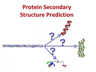
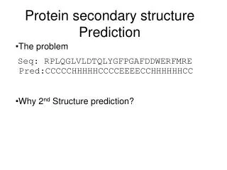
33. Protein secondary structure prediction • Why bother predicting them? • SS Information can be used for downstream analysis: • Framework model of protein folding, collapse secondary structures • Fold prediction by comparing to database of known structures • Can be used as information to predict function • Can also be used to help align sequences (e.g. SS- Praline)

34. Why predict when you can have the real thing? UniProt Release 1.3 (02/2004) consists of:Swiss-Prot Release : 144731 protein sequencesTrEMBL Release : 1017041 protein sequences PDB structures : : ~35000 protein structures Primary structure Secondary structure Tertiary structure Quaternary structure Function ‘Mind the gap’

35. Secondary Structure • An easier question – what is the secondary structure when the 3D structure is known?

36. DSSP • DSSP (Dictionary of Secondary Structure of a Protein) – assignssecondary structure to proteins which have a crystal (x-ray) or NMR (Nuclear Magnetic Resonance) structure H = alpha helix B = beta bridge (isolated residue) E = extended beta strand G = 3-turn (3/10) helix I = 5-turn () helix T = hydrogen bonded turn S = bend DSSP uses hydrogen-bonding structure to assign Secondary Structure Elements (SSEs). The method is strict but consistent (as opposed to expert assignments in PDB

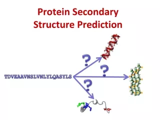
37. A more challenging task:Predicting secondary structure from primary sequence alone

38. What we need to do • Train a method on a diverse set of proteins of known structure • Test the method on a test set separate from our training set • Assess our results in a useful way against a standard of truth • Compare to already existing methods using the same assessment

39. How to develop a method Other method(s) prediction Test set of T<<N sequences with known structure Database of N sequences with known structure Standard of truth Assessment method(s) Method Prediction Training set of K<N sequences with known structure Trained Method

40. Some key features ALPHA-HELIX: Hydrophobic-hydrophilic residue periodicity patterns BETA-STRAND: Edge and buried strands, hydrophobic-hydrophilic residue periodicity patterns OTHER: Loop regions contain a high proportion of small polar residues like alanine, glycine, serine and threonine. The abundance of glycine is due to its flexibility and proline for entropic reasons relating to the observed rigidity in its kinking the main-chain. As proline residues kink the main-chain in an incompatible way for helices and strands, they are normally not observed in these two structures (breakers), although they can occur in the N-terminal two positions of a-helices. Edge Buried

41. Burried and Edge strands Parallel -sheet Anti-parallel -sheet

42. History (1) Using computers in predicting protein secondary has its onset >30 years ago (Nagano (1973) J. Mol. Biol., 75, 401) on single sequences. The accuracy of the computational methods devised early-on was in the range 50-56% (Q3). The highest accuracy was achieved by Lim with a Q3 of 56% (Lim, V. I. (1974) J. Mol. Biol., 88, 857). The most widely used early method was that of Chou-Fasman (Chou, P. Y. , Fasman, G. D. (1974) Biochemistry, 13, 211). Random prediction would yield about 40% (Q3) correctness given the observed distribution of the three states H, E and C in globular proteins (with generally about 30% helix, 20% strand and 50% coil).

43. History (2) Nagano 1973 – Interactions of residues in a window of 6. The interactions were linearly combined to calculate interacting residue propensities for each SSE type (H, E or C) over 95 crystallographically determined protein tertiary structures. Lim 1974 – Predictions are based on a set of complicated stereochemical prediction rules for a-helices and b-sheets based on their observed frequencies in globular proteins. Chou-Fasman 1974 - Predictions are based on differences in residue type composition for three states of secondary structure: a-helix, b-strand and turn (i.e., neither a-helix nor b-strand). Neighbouring residues were checked for helices and strands and predicted types were selected according to the higher scoring preference and extended as long as unobserved residues were not detected (e.g. proline) and the scores remained high.

44. How do secondary structure prediction methods work? • They often use a window approach to include a local stretch of amino acids around a considered sequence position in predicting the secondary structure state of that position • The next slides provide basic explanations of the window approach (for the GOR method as an example) and two basic techniques to train a method and predict SSEs: k-nearest neighbour and neural nets

45. Secondary Structure • Reminder- secondary structure is usually divided into three categories: Anything else – turn/loop Alpha helix Beta strand (sheet)

46. Sliding window Central residue Sliding window Sequence of known structure H H H E E E E • The frequencies of the residues in the window are converted to probabilities of observing a SS type • The GOR method uses three 17*20 windows for predicting helix, strand and coil; where 17 is the window length and 20 the number of a.a. types • At each position, the highest probability (helix, strand or coil) is taken. A constant window of n residues long slides along sequence

47. Sliding window Sliding window Sequence of known structure H H H E E E E • The frequencies of the residues in the window are converted to probabilities of observing a SS type • The GOR method uses three 17*20 windows for predicting helix, strand and coil; where 17 is the window length and 20 the number of a.a. types • At each position, the highest probability (helix, strand or coil) is taken. A constant window of n residues long slides along sequence

48. Sliding window Sliding window Sequence of known structure H H H E E E E • The frequencies of the residues in the window are converted to probabilities of observing a SS type • The GOR method uses three 17*20 windows for predicting helix, strand and coil; where 17 is the window length and 20 the number of a.a. types • At each position, the highest probability (helix, strand or coil) is taken. A constant window of n residues long slides along sequence

49. Sliding window Sliding window Sequence of known structure H H H E E E E • The frequencies of the residues in the window are converted to probabilities of observing a SS type • The GOR method uses three 17*20 windows for predicting helix, strand and coil; where 17 is the window length and 20 the number of a.a. types • At each position, the highest probability (helix, strand or coil) is taken. A constant window of n residues long slides along sequence

50. Chou and Fasman (1974) Name P(a) P(b) P(turn) Alanine 142 83 66 Arginine 98 93 95 Aspartic Acid 101 54 146 Asparagine 67 89 156 Cysteine 70 119 119 Glutamic Acid 151 037 74 Glutamine 111 110 98 Glycine 57 75 156 Histidine 100 87 95 Isoleucine 108 160 47 Leucine 121 130 59 Lysine 114 74 101 Methionine 145 105 60 Phenylalanine 113 138 60 Proline 57 55 152 Serine 77 75 143 Threonine 83 119 96 Tryptophan 108 137 96 Tyrosine 69 147 114 Valine 106 170 50 The propensity of an amino acid to be part of a certain secondary structure (e.g. – Proline has a low propensity of being in an alpha helix or beta sheet  breaker)