Download

1 / 35
350 likes | 521 Vues
Understand the importance of predicting secondary structures in proteins, methods used, role of alignment profiles, and improvements in prediction accuracy. Explore the impact of CASP competition on protein structure prediction.

E N D
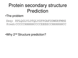
Protein Secondary Structure Prediction G P S Raghava
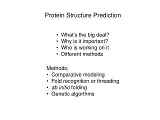
Protein Structure Prediction • Importance • CASP Competition • What is secondary structure • Assignment of secondary structure (SS) • Type of SS prediction methods • Description of various methods • Role of multiple sequence alignment/profiles • How to use
Importance of secondary structure prediction • Classification of protein structures • Definition of loops/core • Use in fold recognition methods • Improvements of alignments • Definition of domain boundaries
CASP changed the landscape • Critical Assessment of Structure Prediction competition. Even numbered years since 1994 • Solved, but unpublished structures are posted in May, predictions due in September • Various categories • Relation to existing structures, ab initio, homology, fold, etc. • Partial vs. Fully automated approaches • Produces lots of information about what aspects of the problems are hard, and ends arguments about test sets. • Results showing steady improvement, and the value of integrative approaches.
CASP Experiment • Experimentalists are solicited to provide information about structures expected to be soon solved • Predictors retrieve the sequence from prediction center (predictioncenter.llnl.gov) • Deposit predictions throughout the season • Meeting held to assess results
Assignment of Secondary Structure • Program • DSSP (Sander Group) • Stride (Argos Group) • Pcurve • DSSP • 3 helix states (I=3,4,5 ) • 2 Sheets (isolated and extended) • Irregular Regions
dssp • The DSSP program defines secondary structure, geometrical features and solvent exposure of proteins, given atomic coordinates in Protein Data Bank format • Usage: dssp [-na] [-v] pdb_file [dssp_file] • Output : 24 26 E H < S+ 0 0 132 25 27 R H < S+ 0 0 125 26 28 N < 0 0 41 27 29 K 0 0 197 28 ! 0 0 0 29 34 C 0 0 73 30 35 I E -cd 58 89B 9 31 36 L E -cd 59 90B 2 32 37 V E -cd 60 91B 0 33 38 G E -cd 61 92B 0
Automatic assignment programs • DSSP ( http://www.cmbi.kun.nl/gv/dssp/ ) • STRIDE ( http://www.hgmp.mrc.ac.uk/Registered/Option/stride.html ) # RESIDUE AA STRUCTURE BP1 BP2 ACC N-H-->O O-->H-N N-H-->O O-->H-N TCO KAPPA ALPHA PHI PSI X-CA Y-CA Z-CA 1 4 A E 0 0 205 0, 0.0 2,-0.3 0, 0.0 0, 0.0 0.000 360.0 360.0 360.0 113.5 5.7 42.2 25.1 2 5 A H - 0 0 127 2, 0.0 2,-0.4 21, 0.0 21, 0.0 -0.987 360.0-152.8-149.1 154.0 9.4 41.3 24.7 3 6 A V - 0 0 66 -2,-0.3 21,-2.6 2, 0.0 2,-0.5 -0.995 4.6-170.2-134.3 126.3 11.5 38.4 23.5 4 7 A I E -A 23 0A 106 -2,-0.4 2,-0.4 19,-0.2 19,-0.2 -0.976 13.9-170.8-114.8 126.6 15.0 37.6 24.5 5 8 A I E -A 22 0A 74 17,-2.8 17,-2.8 -2,-0.5 2,-0.9 -0.972 20.8-158.4-125.4 129.1 16.6 34.9 22.4 6 9 A Q E -A 21 0A 86 -2,-0.4 2,-0.4 15,-0.2 15,-0.2 -0.910 29.5-170.4 -98.9 106.4 19.9 33.0 23.0 7 10 A A E +A 20 0A 18 13,-2.5 13,-2.5 -2,-0.9 2,-0.3 -0.852 11.5 172.8-108.1 141.7 20.7 31.8 19.5 8 11 A E E +A 19 0A 63 -2,-0.4 2,-0.3 11,-0.2 11,-0.2 -0.933 4.4 175.4-139.1 156.9 23.4 29.4 18.4 9 12 A F E -A 18 0A 31 9,-1.5 9,-1.8 -2,-0.3 2,-0.4 -0.967 13.3-160.9-160.6 151.3 24.4 27.6 15.3 10 13 A Y E -A 17 0A 36 -2,-0.3 2,-0.4 7,-0.2 7,-0.2 -0.994 16.5-156.0-136.8 132.1 27.2 25.3 14.1 11 14 A L E >> -A 16 0A 24 5,-3.2 4,-1.7 -2,-0.4 5,-1.3 -0.929 11.7-122.6-120.0 133.5 28.0 24.8 10.4 12 15 A N T 45S+ 0 0 54 -2,-0.4 -2, 0.0 2,-0.2 0, 0.0 -0.884 84.3 9.0-113.8 150.9 29.7 22.0 8.6 13 16 A P T 45S+ 0 0 114 0, 0.0 -1,-0.2 0, 0.0 -2, 0.0 -0.963 125.4 60.5 -86.5 8.5 32.0 21.6 6.8 14 17 A D T 45S- 0 0 66 2,-0.1 -2,-0.2 1,-0.1 3,-0.1 0.752 89.3-146.2 -64.6 -23.0 33.0 25.2 7.6 15 18 A Q T <5 + 0 0 132 -4,-1.7 2,-0.3 1,-0.2 -3,-0.2 0.936 51.1 134.1 52.9 50.0 33.3 24.2 11.2 16 19 A S E < +A 11 0A 44 -5,-1.3 -5,-3.2 2, 0.0 2,-0.3 -0.877 28.9 174.9-124.8 156.8 32.1 27.7 12.3 17 20 A G E -A 10 0A 28 -2,-0.3 2,-0.3 -7,-0.2 -7,-0.2 -0.893 15.9-146.5-151.0-178.9 29.6 28.7 14.8 18 21 A E E -A 9 0A 14 -9,-1.8 -9,-1.5 -2,-0.3 2,-0.4 -0.979 5.0-169.6-158.6 146.0 28.0 31.5 16.7 19 22 A F E +A 8 0A 3 12,-0.4 12,-2.3 -2,-0.3 2,-0.3 -0.982 27.8 149.2-139.1 120.3 26.5 32.2 20.1 20 23 A M E -AB 7 30A 0 -13,-2.5 -13,-2.5 -2,-0.4 2,-0.4 -0.983 39.7-127.8-152.1 161.6 24.5 35.4 20.6 21 24 A F E -AB 6 29A 45 8,-2.4 7,-2.9 -2,-0.3 8,-1.0 -0.934 23.9-164.1-112.5 137.7 21.7 37.0 22.6 22 25 A D E -AB 5 27A 6 -17,-2.8 -17,-2.8 -2,-0.4 2,-0.5 -0.948 6.9-165.0-123.7 138.3 18.9 38.9 20.8 23 26 A F E > S-AB 4 26A 76 3,-3.5 3,-2.1 -2,-0.4 -19,-0.2 -0.947 78.4 -27.2-127.3 111.5 16.4 41.3 22.3 24 27 A D T 3 S- 0 0 74 -21,-2.6 -20,-0.1 -2,-0.5 -1,-0.1 0.904 128.9 -46.6 50.4 45.0 13.4 42.1 20.2 25 28 A G T 3 S+ 0 0 20 -22,-0.3 2,-0.4 1,-0.2 -1,-0.3 0.291 118.8 109.3 84.7 -11.1 15.4 41.4 17.0 26 29 A D E < S-B 23 0A 114 -3,-2.1 -3,-3.5 109, 0.0 2,-0.3 -0.822 71.8-114.7-103.1 140.3 18.4 43.4 18.1 27 30 A E E -B 22 0A 8 -2,-0.4 -5,-0.3 -5,-0.2 3,-0.1 -0.525 24.9-177.7 -74.1 127.5 21.8 41.8 19.1
Secondary Structure Types * H = alpha helix * B = residue in isolated beta-bridge * E = extended strand, participates in beta ladder * G = 3-helix (3/10 helix) * I = 5 helix (pi helix) * T = hydrogen bonded turn * S = bend
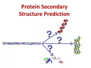
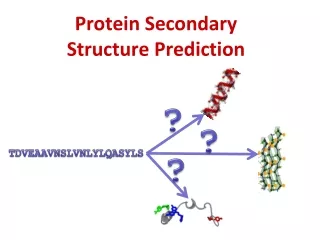
Secondary Structure Prediction • What to predict? • All 8 types or pool types into groups Q3 H * H = a helix * B = residue in isolated b-bridge * E = extended strand, participates in b ladder * G = 3-helix (3/10 helix) E * I = 5 helix (p helix) * T = hydrogen bonded turn * S = bend * C/.= random coil C Straight HEC CASP
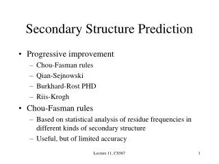
Type of Secondary Structure Prediction • Information based classification • Property based methods (Manual / Subjective) • Residue based methods • Segment or peptide based approaches • Application of Multiple Sequence Alignment • Technical classification • Statistical Methods • Chou & fashman (1974) • GOR • Artificial Itellegence Based Methods • Neural Network Based Methods (1988) • Nearest Neighbour Methods (1992) • Hidden Markove model (1993) • Support Vector Machine based methods
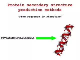
"" בראשית יא א Comparing methods requires same terms and tests. Secondary structure types: H - helix E – β strand L\C – other. seq A A P P L L L L M M M G I M M R R I M E E E E E C C C C H H H H C C C E E E pred
How to evaluate a prediction? The Q3 test: correctly predicted residues number of residues Of course, all methods would be tested on the same proteins.
CHOU- FASMAN ALGORITHM Conformatal parameter: Pα ,Pβand Ptfor each amino acidi Pi,x = f i,x/ < f x > = (n i,x / n i )/ (n x/ N) Nucleation sites and extension Clusters of four helical formers out of six propagated by four residues 4 if < Pα > = ∑ Pα/ 4 1.00 1 Clusters of three β-formers out of five propagated by four residues 4 if < Pβ > = ∑ Pβ / 4 1.00 1 Clusters of four turn residues if Pt = f j ☓ f j+1☓ f j+2☓ f j+3 > 0.75 ☓ 10 –4 Specifics thresholds for < Pα > , < Pβ > and < Pt > and their relatives values decide for the prediction
Amino Acid -Helix -Sheet Turn Ala 1.29 0.90 0.78 Cys 1.11 0.74 0.80 Leu 1.30 1.02 0.59 Met 1.47 0.97 0.39 Glu 1.44 0.75 1.00 Gln 1.27 0.80 0.97 His 1.22 1.08 0.69 Lys 1.23 0.77 0.96 Val 0.91 1.49 0.47 Ile 0.97 1.45 0.51 Phe 1.07 1.32 0.58 Tyr 0.72 1.25 1.05 Trp 0.99 1.14 0.75 Thr 0.82 1.21 1.03 Gly 0.56 0.92 1.64 Ser 0.82 0.95 1.33 Asp 1.04 0.72 1.41 Asn 0.90 0.76 1.23 Pro 0.52 0.64 1.91 Arg 0.96 0.99 0.88 Chou-Fasman Rules (Mathews, Van Holde, Ahern) Favors -Helix Favors -Sheet Favors Turns
Chou-Fasman • First widely used procedure • If propensity in a window of six residues (for a helix) is above a certain threshold the helix is chosen as secondary structure. • If propensity in a window of five residues (for a beta strand) is above a certain threshold then beta strand is chosen. • The segment is extended until the average propensity in a 4 residue window falls below a value. • Output-helix, strand or turn.
GOR method • Garnier, Osguthorpe & Robson • Assumes amino acids up to 8 residues on each side influence the ss of the central residue. • Frequency of amino acids at the central position in the window, and at -1, .... -8 and +1,....+8 is determined for a, b and turns (later other or coils) to give three 17 x 20 scoring matrices. • Calculate the score that the central residue is one type of ss and not another. • Correctly predicts ~64%.
Scoring matrix i-4 i-3 i-2 i-1 i i+1 i+2 i+3 i+4…. T R G Q L I R E A Y E D Y R H F S S E C P F I P
GOR : Information function • Information function, I(Sj;Rj) : • Information that sequence Rj contains about structure Sj • I = 0 : no information • I > 0 : Rj favors Sj • I < 0 : Rj dislikes Sj
GOR: Formulation(1) • Secondary structure should depend on the whole sequence, R • Simplification (1) : only local sequences (window size = 17) are considered • Simplification (2) : each residue position is statistically independent • For independent event, just add up the information
m = +8 I(Sj;R1,R2,…..Rlast) ≃ ∑ I(Sj;Rj+m) m = – 8
Artificial Neural Network What does a neuron do? • Gets “signals” from its neighbours. • Each signal has different weight. • When achieving certain threshold - sends signals.
Architecture Weights Input Layer I K H Output Layer E E E C H V I I Q A E Hidden Layer Window IKEEHVIIQAEFYLNPDQSGEF…..
Artificial Neural Network General structure of ANN : • One input layer. • Some hidden layers. • One output layer. • Our ANN have one-direction flow !
Secondary Structure Prediction • Application of Multiple sequence alignment • Segment based (+8 to -8 residue) • Input Multiple alignment instead of single seq uence • Application of PSIBLAST • Current methods (combination of) • Segment based • Neural network • Multiple sequence alignment (PSIBLAST) • Combination of Neural Network + Nearest Neighbour Method
Structure of 3rd generation methods Find homologues using large data bases. Create a profile representing the entire protein family. Give sequence and profile to ANN. Output of the ANN: 2nd structure prediction.
PSI - PRED Reliability numbers: • The way the ANN tells us • how much it is sure about • the assignment. • Used by many methods. • Correlates with accuracy.
Performance evaluation • Through 3rd generation methods accuracy • jumped ~10%. • Many 3rd generation methods exist today. Which method is the best one ? How to recognize “over-optimism” ?
PSIPRED • Uses multiple aligned sequences for prediction. • Uses training set of folds with known structure. • Uses a two-stage neural network to predict structure based on position specific scoring matrices generated by PSI-BLAST (Jones, 1999) • First network converts a window of 15 aa’s into a raw score of h,e (sheet), c (coil) or terminus • Second network filters the first output. For example, an output of hhhhehhhh might be converted to hhhhhhhhh. • Can obtain a Q3 value of 70-78% (may be the highest achievable)