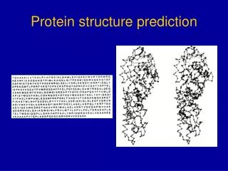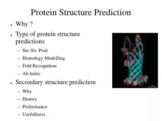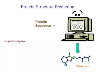
Protein structure prediction

1. Protein structure prediction • May 15, 2001 • Quiz#4 postponed • Writing assignment • Learning objectives-Understand the basis of secondary structure prediction programs. Understand neural networks. Become familiar with manipulating known protein structures with Cn3D. • Workshop-Manipulation of the PTEN protein structure with Cn3D.

2. What is secondary structure? • Two major types: • Alpha Helical Regions • Beta Sheet Regions • Other classification schemes: • Turns • Transmembrane regions • Internal regions • External regions • Antigenic regions

3. Some Prediction Methods • ab initio methods • Based on physical properties of aa’s and bonding patterns • Statistics of amino acid distributions • Chou-Fasman • Position of amino acid and distribution • Garnier, Osguthorpe-Robeson (GOR) • Neural networks

4. Chou-Fasman Rules (Mathews, Van Holde, Ahern Amino Acid -Helix -Sheet Turn Ala 1.29 0.90 0.78 Cys 1.11 0.74 0.80 Leu 1.30 1.02 0.59 Met 1.47 0.97 0.39 Glu 1.44 0.75 1.00 Gln 1.27 0.80 0.97 His 1.22 1.08 0.69 Lys 1.23 0.77 0.96 Val 0.91 1.49 0.47 Ile 0.97 1.45 0.51 Phe 1.07 1.32 0.58 Tyr 0.72 1.25 1.05 Trp 0.99 1.14 0.75 Thr 0.82 1.21 1.03 Gly 0.56 0.92 1.64 Ser 0.82 0.95 1.33 Asp 1.04 0.72 1.41 Asn 0.90 0.76 1.23 Pro 0.52 0.64 1.91 Arg 0.96 0.99 0.88 Favors -Helix Favors -Sheet Favors -Sheet

5. Chou-Fasman • First widely used procedure • If propensity in a window of six residues (for a helix) is above a certain threshold the helix is chosen as secondary structure. • If propensity in a window of five residues (for a beta strand) is above a certain threshold then beta strand is chosen. • The segment is extended until the average propensity in a 4 residue window falls below a value. • Output-helix, strand or turn.

6. GOR Position-dependent propensities for helix, sheet or turn is calculated for each amino acid. For each position j in the sequence, eight residues on either side of aaj is considered. It uses a PSSM A helix propensity table contains info. about propensity for certain residues at 17 positions when the conformation of residue j is helical. The helix propensity tables have 20 x 17 entries. The predicted state of aaj is calculated as the sum of the position-dependent propensities of all residues around aaj.

7. Neural networks • Computer neural networks are based on simulation of adaptive • learning in networks of real neurons. • Neurons connect to each other via synaptic junctions which are either • stimulatory or inhibitory. • Adaptive learning involves the formation or suppression of the right • combinations of stimulatory and inhibitory synapses so that a set • of inputs produce an appropriate output.

8. Neural Networks (cont. 1) • The computer version of the neural network involves • identification of a set of inputs - amino acids in the • sequence, which transmit through a network of • connections. • At each layer, inputs are numerically • weighted and the combined result passed to the next • layer. • Ultimately a final output, a decision, helix, sheet or • coil, is produced.

9. Neural Networks (cont. 2) 90% of training set was used (known structures) 10% was used to evaluate the performance of the neural network during the training session.

10. Neural Networks (cont. 3) • During the training phase, selected sets of proteins of known structure are scanned, and if the decisions are incorrect, the input weightings are adjusted by the software to produce the desired result. • Training runs are repeated until the success rate is maximized. • Careful selection of the training set is an important aspect of this technique. The set must contain as wide a range of different fold types as possible, but without duplications of structural types that may bias the decisions.

11. Neural Networks (cont. 5) • An additional component of the PSIPRED procedures involves sequence alignment with similar proteins. • The rationale is that some amino acids positions in a sequence contribute more to the final structure than others. (This has been demonstrated by systematic mutation experiments in which each consecutive position in a sequence is substituted by a spectrum of amino acids. Some positions are remarkably tolerant of substitution, while others have unique requirements.) • To predict secondary structure accurately, one should place little weight on the tolerant positions, which clearly contribute little to the structure, and strongly emphasize the intolerant positions.

12. PSIPRED • Uses multiple aligned sequences for prediction. • Uses training set of proteins with known structure. • Uses a two-stage neural network to predict structure based on position specific scoring matrices generated by PSI-BLAST (Jones, 1999) • First network converts a window of 15 aa’s into a raw score of h,b,c or terminus • Second network filters the first output. For example, an output of hhhhehhhh might be converted to hhhhhhhhh. • Can obtain a Q3 value of 70-78% (may be the highest achievable)

13. Provides info on tolerant or intolerant positions Column specifies position within the protein 15 groups of 21 units (1 unit for each aa plus one specifying the end) Filtering network three outputs are helix, strand or coil

14. Example of Output from PSIPRED PSIPRED PREDICTION RESULTS Key Conf: Confidence (0=low, 9=high) Pred: Predicted secondary structure (H=helix, E=strand, C=coil) AA: Target sequence Conf: 923788850068899998538983213555268822788714786424388875156215 Pred: CCEEEEEEEHHHHHHHHHHCCCCCCHHHHHHCCCCCEEEEECCCCCCHHHHHHHCCCCCC AA: KDIQLLNVSYDPTRELYEQYNKAFSAHWKQETGDNVVIDQSHGSQGKQATSSVINGIEAD 10 20 30 40 50 60

15. 3D structure prediction-Threading Threading, alluded to earlier, is a mechanism to address the alignment of two sequences that have <30% identity and are typically considered non-homologous. Essentially, one fits—or threads—the unknown sequence onto the known structure and evaluates the resulting structure’s fitness using environment- or knowledge-based potentials.

16. Helical Wheel If you can predict an alpha helix it is sometimes useful to be able to tell if the helix is amphipathic. This would indicate whether one face of the helix faces the solvent or perhaps another protein. They have been particularly useful in predicting a “super-secondary” structure known as coiled coils. The helical wheel is based on the ideal alpha helix placing an amino acid every 100* around the circumference of the helix cylinder

17. Coiled-coil predictors The alpha-helical coiled-coil structure has a strong signature heptad pattern abcdefg where a and d are typically non polar (leucine rich) and e and g are often charged. This makes scoring from a sequence scale plot relatively easy.

18. 3D structure data • The largest 3D structure database is the Protein Database • It contains over 15,000 records • Each record contains 3D coordinates for macromolecules • 80% of the records were obtained from X-ray diffraction studies, 16% from NMR and the rest from other methods and theoretical calculations

19. Part of a record from the PDB ATOM 1 N ARG A 14 22.451 98.825 31.990 1.00 88.84 N ATOM 2 CA ARG A 14 21.713 100.102 31.828 1.00 90.39 C ATOM 3 C ARG A 14 22.583 101.018 30.979 1.00 89.86 C ATOM 4 O ARG A 14 22.105 101.989 30.391 1.00 89.82 O ATOM 5 CB ARG A 14 21.424 100.704 33.208 1.00 93.23 C ATOM 6 CG ARG A 14 20.465 101.880 33.215 1.00 95.72 C ATOM 7 CD ARG A 14 20.008 102.147 34.637 1.00 98.10 C ATOM 8 NE ARG A 14 18.999 103.196 34.718 1.00100.30 N ATOM 9 CZ ARG A 14 18.344 103.507 35.833 1.00100.29 C ATOM 10 NH1 ARG A 14 18.580 102.835 36.952 1.00 99.51 N ATOM 11 NH2 ARG A 14 17.441 104.479 35.827 1.00100.79 N

20. Molecular Modeling DB (MMBD) • Relies on PDB for data • It contains over 10,000 structure records • Links connect the records to Medline and NCBI’s taxonomy database • Sequence “neighbors” of the structures are are provided by BLAST. • Structure “neighbors” are provided by VAST algorithm. • Cn3D is a molecular graphics viewer that allows one to view the three-dimensional structure.