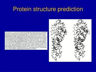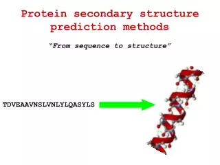
Chapter 14 Protein Secondary Structure Prediction
Chapter 14 Protein Secondary Structure Prediction. Refresher. Proteins have secondary structures These structures are essential to maintain the 3D structure of the protein Secondary structure can be either of -helix -strand Coil

Chapter 14 Protein Secondary Structure Prediction
E N D
Presentation Transcript
Chapter 14 Protein Secondary Structure Prediction
Refresher • Proteins have secondary structures • These structures are essential to maintain the 3D structure of the protein • Secondary structure can be either of • -helix • -strand • Coil • -helix H-bond between C=O and N-H of every 4+ith residue • 3.6 aa per turn • 1.5 Å / aa (= 5.4 Å per turn) • (fully extended peptide backbone = 3.5 Å / aa) • -strand H-bond between C=O and N-H of distant regions • Parallel or anti-parallel • Coiled coil • Hydrophobic amino acids interact
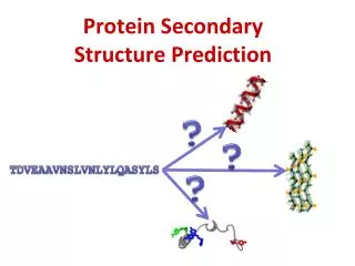
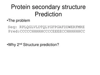
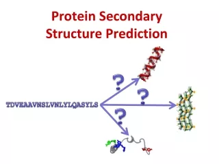
Secondary Structure Predictions • Prediction of conformation of each amino acid: • H: -helix • E: -strand • C: Coil (no defined 2° structure) • Used for classification of proteins • Defining domains and motifs • Intermediary step towards 3° structure prediction • Globular and trans-membrane proteins are structurally very different • Required different algorithms to predict these two classes of proteins
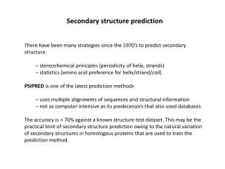
Problem is not trivial • -helix based on short distance (4+i interactions) • -strand based on long distance (5 – 50+ residues) • Long range interaction predictions less accurate • Accuracy about 75% • Ab initio based • Statistical calculation of residues in single query sequence • Homology-based • Common 2° structure patterns in homologous sequences
Ab initio Methods Chou-Fasman Intrinsic property of residue to be in helix, strand or turn structure A, E, M common in -helices N: residues in all protein structures M: residues in -helices Y: Total Ala in protein structures X: Ala in -helices Propensity Ala in -helix: (X/Y)/(M/N) Value = 1: same distribution as average Value > 1: more often in -helix than average Value < 1: less often in -helix than average 6 residue window of which 4 is H -helix Window extended bidirectionally until P < 1.0 5 residue window of which 3 is E -strand
http://fasta.bioch.virginia.edu/fasta_www2/fasta_www.cgi?rm=misc1http://fasta.bioch.virginia.edu/fasta_www2/fasta_www.cgi?rm=misc1
Example Chou-Fasman 10 20 30 40 50 60 SRRSASHPTY SEMIAAAIRA EKSRGGSSRQ SIQKYIKSHY KVGHNADLQI KLSIRRLLAA 70 80 90 GVLKQTKGVG ASGSFRLAKS DKAKRSPGKK HELIX 1 HA1 SER A 29 ALA A 38 HELIX 2 HA2 ARG A 47 SER A 56 HELIX 3 HA3 ALA A 64 ALA A 78 SHEET 1 SA 3 SER A 45 SER A 46 SHEET 2 SA 3 GLY A 91 ARG A 94 SHEET 3 SA 3 LEU A 81 GLY A 86 . . . . . . SRRSASHPTYSEMIAAAIRAEKSRGGSSRQSIQKYIKSHYKVGHNADLQIKLSIRRLLAA helix <--------> <-----> <----------------- sheet EEEEEEEEE EEEEEE EEEEEEEEEEEEE turns T T T T T . . . GVLKQTKGVGASGSFRLAKSDKAKRSPGKK helix -------> <-------> sheet EEEEEEEEE turns T T TT T
Garnier-Osguthorpe-Robson (GOR) • Makes use of distant influences on propensity • Uses 17 residue window • Adds propensity for four 2º structure states (H, E, T, C) • Highest value defines 2º structure state of central residue in window . 10 . 20 . 30 . 40 . 50 . 60 SRRSASHPTYSEMIAAAIRAEKSRGGSSRQSIQKYIKSHYKVGHNADLQIKLSIRRLLAA helix HHHHHHHHHHH HHHHHH HHHH sheet EEEEEEEE E EEEEEE turns TTTT TTTTT T TTTT coil C CCCCC CCC C . 70 . 80 . 90 GVLKQTKGVGASGSFRLAKSDKAKRSPGKK helix HHHH HHHHHHHHHHH sheet EEEEE E turns TTT coil CCCC C C Residue totals: H: 36 E: 21 T: 17 C: 16 percent: H: 48.6 E: 28.4 T: 23.0 C: 21.6
Expansion using larger crustal structure databases • Algorithms based on a larger database of crystal structure information: • GOR II, III and IV • SOPM • http://npsa-pbil.ibcp.fr/cgi-bin/npsa_automat.pl?page=/NPSA/npsa_server.html SRRSASHPTYSEMIAAAIRAEKSRGGSSRQSIQKYIKSHYKVGHNADLQIKLSIRRLLAAGVLKQTKGVG cccccccchhhhhhhhhhhhtccttcccchhhhhhhhhtcccccccthhhhhhhhhhhhhhhhhttttcc ASGSFRLAKSDKAKRSPGKK cccceeeecccccccccccc
Neural Network programs • A neural net has an input layer, hidden layers composed of nodes given different weights, and an output layer • Neural net trained with multiply aligned sequences • Accuracy >75% • PHD • BLASTP • MAXHOM (sequence alignment) • Neural Net • Layer one : 13 residue window • Layer two: 17 residue window • Layer three: “Jury layer” – removes very short stretches • PSIPRED • PSI-BLAST • Neural net • SSpro • PROTER • PROF • HMMSTR
Predictions with Multiple Methods • No single prediction program is correct, and it is generally good practice to use the output from several programs • Some web servers do this: • JPred • PHD, PREDATOR, DSC, NNSSP, Inet and ZPred • First submitted to PSI-BLAST • Multiple alignment • Submitted to above 6 programs • Consensus returned • No consensus, uses PHD • SRRSASHPTYSEMIAAAIRAEKSRGGSSRQSIQKYIKSHYKVGHNADLQIKLSIRRLLAAGVLKQTKGVGASGSFRLAKSDKAKRSPGKK • ---------HHHHHHHHHHH--------HHHHHHHHHH-------HHHHHHHHHHHHH---EEEEE------EEEE--------------
Trans-membrane proteins • Two types of trans-membrane proteins • -helix • -barrel • Many consists solely of -helix and are found in the cytoplasmic membrane • -barrel normally found in outer-membrane of gram negative bacteria • Difficult to get X-ray or NMR structure
-helix perpendicular to membrane 17-25 residues • Hydrophobic residues separated by hydrophilic loops (<60 residues) • Residues bordering hydrophobic module is generally charged • Inner cytosolic region most often highly charged (orientation info) • Positive inside rule • Scan window 17-25 residues calculate hydrophobicity score • Many false positives • Signal peptide sequences confuse algorithm
TMHMM • Trained with 160 known TM sequences • Probability of having an -helix is given • Orientation of -helix based on positive inside rule • Phobius • Incorporates distinct HMM models for signal peptides and TM helices • Signal peptide sequence ignored • Can use sequence homologs and multiply aligned sequences
Prediction of -barrel proteins • -strand forming trans-membrane section is amphipatic • 10-22 residues • Alternating hydrophobic and hydrophilic sequence arrangement • -helix TM prediction programs thus not applicable to -barrel proteins • TBBpred • Neural net trained with -barrel protein sequences
Coiled coil prediction • Two or more -helices winding around each other • For every 7 residues, 1 and 4 are hydrophobic, facing central core • Coils • Scan window of 14, 21 or 28 residues • Compares residues to probability matrix based on known coiled coils • Accurate for left-handed coil, but not right-handed coil • Multicoil • Scoring matrix based on 2-strand and 3-strand coils • Used in several genome-wide studies • Leucine zippers • sub-class of coiled coils • L-X6-L-X6-L- • Found in transcription factors • Anti-parallel -helices stabilized by leucine core
Chapter 13 Protein Tertiary Structure Prediction
The need for predicting 3D structures • X-ray crystallography is extremely tedious • DNA sequences and therefore protein sequences are rapidly generated • A gap between sequence and structure is widening • Protein structure often provides insight info function • Thee main methods for 3D prediction • Homology modeling • Threading • Ab initio
Template Selection • Search PDB for homologous sequences with BLAST or FASTA • Should have >30% sequence identity (20% at a stretch) • In case of multiple hits, choose • Highest identity • Highest resolution • Most appropriate co-factors Sequence Alignment Critical Incorrectly aligned residues will give an incorrect model Use Praline or T-Coffee for alignment Inspect visually to confirm alignment of key residues
Backbone Model Building • Copy the backbone atoms of the query sequence to that of the corresponding aligned residue • If the residues are identical, the coordinates of the whole residue can be copied • If the residues are different, only the C are copied • The remaining atoms of the residue are modeled later Loop Modeling • It often happens that there are “gaps” in the aligned sequences • Two techniques to connect the protein on either side of the gap: • Database • Search database for fragments that fit the gap • Measure coordinates and orientation of backbone on either side of gap • Search for fragments that can fit • Best loop gives no steric clash with structure • Ab Initio • Generate random loop No clash with nearby side-chains • And angles in acceptable region of Ramachandran plot
Side Chain Refinement • Need to model side-chains where these differ from aligned template sequence • Search database for all occurrences of given side-chain in backbone conformation and minimal clash with neighbouring residues • Computationally prohibitive • Library of rotamers • Collection of conformations for each residue that is most often observed in structure database • Select rotamer with conformation that best fits backbone • Minimal interference with neighbouring side-chains • SCWRL
Model Refinement using Energy Function • After loop modeling and side-chain refinement the follwing remain • Unfavourable torsion angles • Unacceptable proximity of atoms • Use energy minimization to alleviate such problems • Limit number of iteration (<100) to ensure that the entire model does not change form the template • Molecular Dynamic can be used to search for a global minimum Model Evaluation • Check consistency in - angles • Bond lengths • Close contacts • Flag regions below acceptability threshold • Procheck • WHATIF • ANOLEA • Verify3D
Comprehensive Modeling Programs • Modeler • Swiss-Model • 3D-Jigsaw
Threading and Fold Recognition • Pairwise Energy Method • Fit sequence to each fold in database • Use local alignment to improve fit • Calculate energies • Pairwise residue interaction • Solvation Hydrophobic • Profile Method • Fit sequence to fold • Calculate propensity of each amino acid to be present at each profile position • Secondary structure types • Solvent exposure • Hydrophobicity • Use structure fold that best fits profile of parameters
Ab Initio Prediction Protein fold into a native, low-energy native state The mechanism driving this process is poorly understood Computationally untenable to explore all possible states and calculate energies A 40 residue peptide will require 1020 years to calculate all states using a 1×10¹² FLOPS computer Not realistic approach currently