Download
1 / 16
160 likes | 326 Vues
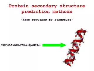
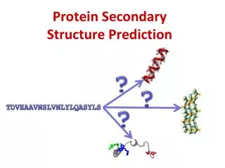
Secondary Structure Prediction. Progressive improvement Chou-Fasman rules Qian-Sejnowski Burkhard-Rost PHD Riis-Krogh Chou-Fasman rules Based on statistical analysis of residue frequencies in different kinds of secondary structure Useful, but of limited accuracy. Qian-Sejnowski.

E N D
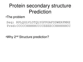
Secondary Structure Prediction • Progressive improvement • Chou-Fasman rules • Qian-Sejnowski • Burkhard-Rost PHD • Riis-Krogh • Chou-Fasman rules • Based on statistical analysis of residue frequencies in different kinds of secondary structure • Useful, but of limited accuracy Lecture 11, CS567
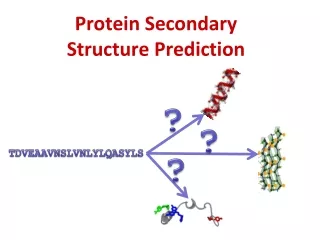
Qian-Sejnowski • Pioneering NN approach • Input: 13 contiguous amino acid residues • Output: Prediction of secondary structure of central residue • Architecture: • Fully connected MLP • Orthogonal encoding of input, • Single hidden layer with 40 units • 3 neuron output layer • Training: • Initial weight between -0.3 and 0.3 • Backpropagation with the LMS (Steepest Descent) algorithm • Output: Helix xor Sheet xor Coil (Winner take all) Lecture 11, CS567
Qian-Sejnowski • Performance • Dramatic improvement over Chou-Fasman • Assessment • Q = 62.7% (Proportion of correct predictions) • Correlation coefficient (Eq 6.1) • Better parameter because • It considers all of TP, FP, TN and FN • Chi-squared test can be used to assess significance • C = 0.35; C = 0.29, Cc = 0.38; • Refinement • Outputs as inputs into second network (13X3 inputs, otherwise identical) • Q = 64.3%; C = 0.41; C = 0.31, Cc = 0.41 Lecture 11, CS567
PHD (Rost-Sander) • Drawback of QS method • Large number of parameters (104 versus 2 X 10⁴ examples) leads to overfitting • Theoretical limit on accuracy using only sequence per se as input~ 68% • Key aspect of PHD: Use evolutionary information • Go beyond single sequence by using information from similar sequences (Enhance signal-noise ratio; “Look for more swallows before declaring summer”) through multiple sequence alignments • Prediction in context of conservation (similar residues) within families of proteins • Prediction in context of whole protein Lecture 11, CS567
PHD (Rost-Sander) • Find proteins similar to the input protein • Construct a multiple sequence alignment • Use frequentist approach to assess position-wise conservation • Include extra information (similarity) in the network input • Position-wise conservation weight (Real) • Insertion (Boolean); Deletion (Boolean) • Overfitting minimized by • Early stopping and • Jury of heterogeneous networks for prediction • Performance • Q = 69.7%; C = 0.58; C = 0.5, Cc = 0.5 Lecture 11, CS567
PHD inputFig 6.2 Lecture 11, CS567
PHD architectureFig 6.2 Lecture 11, CS567
Riis-Krogh NN • Drawback of PHD • Large input layer • Network globally optimized for all 3 classes; scope for optimizing wrt each predicted class • Key aspects of RK • Use local encoding with weight sharing to minimize number of parameters • Different network for prediction of each class Lecture 11, CS567
RK architecture (Fig 6.3) Lecture 11, CS567
RK architecture (Fig 6.4) Lecture 11, CS567
Riis-Krogh NN • Find proteins similar to the input protein • Construct a multiple sequence alignment • Use frequentist approach to assess position-wise conservation • BUT first predict structure of each sequence separately, followed by integration based on conservation weights Lecture 11, CS567
Riis-Krogh NN • Architecture • Local encoding • Each amino acid represented by analog value (‘real correlation’, not algebraic) • Weight sharing to minimize parameters • Extra hidden layer as part of input • For helix prediction network, use sparse connectivity based on known periodicity • Use ensembles of networks differing in architecture for prediction (hidden units) • Second integrative network used for prediction • Performance • Q = 71.3%; C = 0.59; C = 0.5, Cc = 0.5 • Corresponds to theoretical upper bound for a contiguous window based method Lecture 11, CS567
NN tips & tricks • Avoid overfitting (avoid local minima) • Use the fewest parameters possible • Transform/filter input • Use weight sharing • Consider partial connectivity • Use large number of training examples • Early stopping • Online learning as opposed to batch/offline learning (“One of the few situations where noise is beneficial”) • Start with different values for parameters • Use random descent (“ascent”) when needed Lecture 11, CS567
NN tips & tricks • Improving predictive performance • Experiment with different network configurations • Combine networks (ensembles) • Use priors in processing input (Context information, non-contiguous information) • Use appropriate measures of performance (e.g., correlation coefficient for binary output) • Use balanced training • Improving computational performance • Optimization methods based on second derivatives Lecture 11, CS567
Measures of accuracy • Vector of TP, FP, TN, FN is best, but not very intuitive measure of distance between data (target) and model (prediction), and restricted to binary output • Alternative: Single measures (transformation of above vector) • Proportions based on TP, FP, TN, FN • Sensitivity (Minimize false negatives) • Specificity (Minimize false positives) • Accuracy (Minimize wrong predictions) Lecture 11, CS567
Measures of error/accuracy • Lp distances (Minkowski distances) • (i |di - mi|p )1/p • L1 distance = Hamming/Manhattan distance = i |di - mi| • L2 distance = Euclidean/Quadratic distance = (i |di - mi|2 )1/2 • Pearson correlation coefficient • I (di – E[d])(mi - E[m])/d m • (TP.TN – FP.FN)/(TP+FN)(TP+FP)(TN+FP)(TN+FN) • Relative entropy (déjà vu) • Mutual information (déjà vu aussi) Lecture 11, CS567