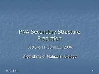
RNA Secondary Structure Prediction

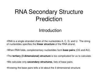
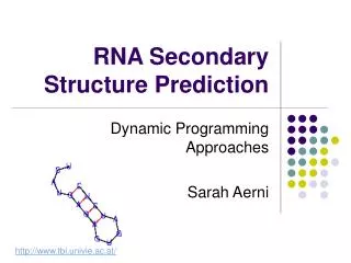
1. RNA Secondary Structure Prediction • RNA is a single-stranded chain of the nucleotides A, C, G, and U. The string of nucleotides specifies the linear structure of the RNA strand. • When RNA folds, complementary nucleotides form base pairs (CG and AU). • The tertiary (3 dimensional) structure is too complicated for us to calculate. • We calculate only secondary structures, lists of base pairs. • Knowing the base pairs tells a lot about the 3 dimensional structure. Introduction

2. Chemical Structure of RNA • Four base types. • Distinguishable ends.

3. Partial Tertiary Structure • One illustration

4. Yet Another Tertiary Structure • Found via google

5. Our Final Tertiary Picture • Very complex

6. A Partial RNA Secondary Structure

7. Pure Secondary Structure

8. Our Basic Model • RNA linear structure: R=r1 r2 . . . rn from {A,C,G,U} • RNA secondary structure: pairs (ri,rj) such that 0<i<j<n+1. • Goal: secondary structures with minimum free energy.

9. Implementing Model Restrictions • No knots: pairs (ri,rj) and (rk,rl) such that i<k<j<l. RNA does contain knots. • Program loop structure. • No “close” base pairs: j-i>t for some t>0. • High free energy. • Complementary base pairs: A-U, C-G. • High free energy.

10. Our Two Algorithms • Independent base pairs – quite easy, but inaccurate. • Calculate loops’ free energy – best we can do for today’s class.

11. Independent Base Pair Algorithm • Assumption: Independent base pairs. • Advantage 1: Simpler calculations. • Advantage 2: Illustrates ideas for a much more accurate algorithm. • Disadvantage: Unrealistic answers.

12. Independent Base PairsWhat Makes It “Easy”? • Assumption: The energy of each base pair is independent of all of the other pairs and the loop structure. • Consequence: Total free energy is the sum of all of the base pair free energies.

13. Independent Base PairsBasic Approach • Use solutions for smaller strings to determine solutions for larger strings. • This is precisely the kind of decoupling required for dynamic programming algorithms to work.

14. Independent Base Pairs Notation • a(ri,rj) – the free energy of a base pair joining ri and rj. • Si,j – The secondary structure of the RNA strand from base ri to base rj. Ie, the set of base pairs between ri and rj inclusive. • E(Si,j) – The free energy associated with the secondary structure Si,j. • We define a(ri,rj) large when constraints are violated.

15. Independent Base Pairs:Calculating Free Energy • Consider the RNA strand from position i to j. • Consider whether rj is paired • If rj is paired, E(Si,j)=E(Si,k-1)+a(k,j)+E(Sk+1,j-1) for some i-1<k<j • If rj isn’t paired, then E(Si,j)=E(Si,j-1)

16. Independent Base Pairs - Algorithm • We search for intervals with minimum free energy. • For each interval, the free energy is given by this formula: E(Si,j) = min( E(Si+1,j-1)+a(ri,rj), E(Si,k-1+a(ri,rk)+Sk+1,j-1), i -1<k<j+1 ) • The free energy of the RNA strand is E(S1,n).

17. Independent Base Pairs:Question 1 • How does this formula deal with the case where rj isn’t paired with any base? • A special case of E(Si,k-1+a(ri,rk)+Sk+1,j-1), i -1<k<j+1 • The special case with k=j.

18. Independent Base Pairs:Question 2 • What is the high level algorithm flow? • Advance from smaller to larger intervals, calculating free energy costs. • Trace back the path that corresponds to the maximum free energy cost.

19. Independent Base Pairs:Question 3 • In what orders can the intervals’ free energy costs be evaluated? • Major = lower, minor = upper bound • Major = upper, minor = lower bound • Diagonally • Any order (eg, random) that respects the partial order induced by inclusion

20. Independent Base Pairs:Question 4 • What are the time and storage requirements of this algorithm? • Express your answer in terms of the number of bases in the RNA strand. • Since the number of intervals is quadratic, the storage requirements are quadratic. • Since the time requirement for each interval is linear, total time is cubic.

21. Independent Base Pairs: Question 5 • Why not simply calculate free energies as they are needed? Why store them at all? • Because the recursive calls would turn our polynomial algorithm into an exponential algorithm.

22. Independent Base Pairs:Question 6 • How does traceback work for this algorithm? • Recalculate which subinterval yields the maximum free energy. • Save traceback paths.

23. Loop Free Energy Algorithm • An RNA molecule’s free energy is not independent of all other base pairs. • An RNA molecules free energy actually depends on its loop structure. • What do we mean by loops?

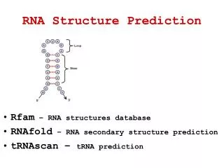
24. Types of Loops • Each base pair (ri,rj) encloses a loop: • Hairpin loop • Bulge on i or j • Interior loop • Helical region

25. Hairpin Loop • There are no base pairs (rk,rl) for i<k<l<j.

26. Bulge on i and j • Bulge on i: • (ri,rj) and (rk,rj-1) are base pairs with k>i+1. • ri+1 is not paired. • The bulge on j is symmetric.

27. Interior loop • (ri,rj) and (rk,rl) are base pairs with i+1<k1<k2<j-1. • ri+1 and rj-1 are not in base pairs

28. Helical region • (ri,rj) and (ri+1,rj-1) are base pairs.

29. Free energy analysis • E(Si,j) = E(Si+1,j) when ri isn’t paired. • E(Si,j) = E(Si,j-1) when rj isn’t paired. • E(Si,j) = min(E(Si,k)+E(Sk+1,j)) for i<k<l, k between i’s and j’s pairs when i and j are paired but not to each other • E(Si,j) = E(Li,j) where Li,j is loop energy when I and j are paired to each other

30. Free Energy Functions • a(ri,rj) – Free energy of base pair (ri,rj) • H(k) – Destabilizing free energy of a hairpin loop with size k. • R – Stabilizing free energy of adjacent base pairs (helical region). • B(k) – Destabilizing free energy of a bulge of size k. • I(k) – Destabilizing free energy of an interior loop of size k.

31. Loop Energy Formulas • H(j-i-1) – for a hairpin loop • R + E(Si+1,j-1) – for a helical region • B(k) + E(Si+k+1,j-1) – for a bulge on i • B(k) + E(Si+1,j-k-1) – for a bulge on j • I(k1+k2) + E(Si+k1+1,j-k2-1) – for an interior loop

32. Free Energy Calculationfor interval (i,j) • Minimize over • Case where (ri,rj) is not a pair. • Case where (ri,rj) is a pair. • Add a(ri,rj) to the formulas. • Minimize over k, k1, and k2.

33. What is the Apparent Complexity? • The interior loop calculations are given by I(k1+k2) + E(Si+k1+1,j-k2-1) • The number of inner loop possibilities is quadratic in the interval size. • The number of intervals is quadratic in the size of the problem. • The complexity appears to grow as n4.

34. What is the Actual Complexity? • Overall reduction from n4 to n3 is possible. • Interval reduction from n2 to linear. • Store the minimum free energy Vi,j,k where the interval (i,j) contains an interior loop of size k.

35. Multiple Solutions • Care must be taken to define the issues. • Multiple solutions can be obtained by adding flexibility to the traceback logic. • The number of solutions can grow exponentially.

36. References • M. Zuker, “The Use of dynamic programming in RNA secondary structure prdiction”. In M. S. Waterman, editor, Mathematical Methods for DNS Sequences. Boca Raton, FL: CRC Press, 1989 • J, Setubal and J. Meidanis,Ch 8.1, Introduction to Computational Molecular Biology, Pacific Grove, CA: Brooks/Cole Publishing Co., 1997