RNA secondary structure
6.096 – Algorithms for Computational Biology. RNA secondary structure. Lecture 1 - Introduction Lecture 2 - Hashing and BLAST Lecture 3 - Combinatorial Motif Finding Lecture 4 - Statistical Motif Finding Lecture 5 - Sequence alignment and Dynamic Programming. 8. 2. 6. 9. 5. 7. 1.


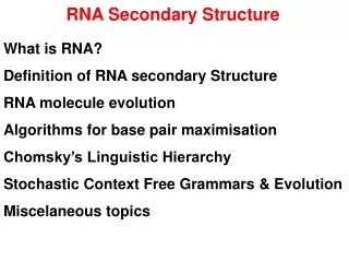
RNA secondary structure
E N D
Presentation Transcript
6.096 – Algorithms for Computational Biology RNA secondary structure Lecture 1 - Introduction Lecture 2 - Hashing and BLAST Lecture 3 - Combinatorial Motif Finding Lecture 4 - Statistical Motif Finding Lecture 5 - Sequence alignment and Dynamic Programming
8 2 6 9 5 7 1 Challenges in Computational Biology 4 Genome Assembly Regulatory motif discovery Gene Finding DNA Sequence alignment Comparative Genomics TCATGCTAT TCGTGATAA TGAGGATAT TTATCATAT TTATGATTT 3 Database lookup Evolutionary Theory RNA folding Gene expression analysis RNA transcript 10 Cluster discovery 11 Gibbs sampling 12 Protein network analysis 13 Regulatory network inference 14 Emerging network properties
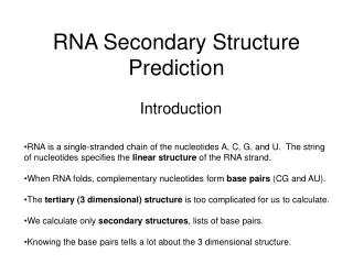
RNA RNA-mediated Replication Self-modification RNA RNA Folding RNA The world before DNA or Protein
RNA World • RNA can be protein-like • Ribozymes can catalyze enzymatic reactions by RNA secondary fold • Small RNAs can play structural roles within the cell • Small RNAs play versatile roles in gene regulatory • RNA can be DNA-like • Made of digital information, can transfer to progeny by complementarity • Viruses with RNA genomes (single/double stranded) • RNA can catalyze RNA replication • RNA world is possible • Proteins are more efficient (larger alphabet) • DNA is more stable (double helix, less flexible)
RNA invented its successors • RNA invents protein • Ribosome precise structure was solved this past year • Core is all RNA. Only RNA makes DNA contact • Protein component only adds structural stability • RNA and protein invent DNA • Stable, protected, specialized structure (no catalysis) • Proteins catalyze: RNADNA reverse transcription • Proteins catalyze: DNADNA replication • Proteins catalyze: DNARNA transcription • Viruses still preserved from those early days of life • Any type genome: dsDNA, ssRNA, dsRNA, hybrid • Simplest self-replicating life form
Example: tRNA secondary and tertiary structure Primary Structure Tertiary Structure Secondary Structure Adaptor molecule between DNA and protein
Hairpin Loops Interior loops Stems Multi-branched loop Bulge loop Most common folds
More complex folds Kissing Hairpins Pseudoknot Hairpin-bulge interaction
Dynamic programming algorithmfor secondary structure determination
First DP Algorithm: Nussinov • one possible technique: base pair maximization • Algorithms for Loop Matching(Nussinov et al., 1978) • too simple for accurate prediction, but stepping-stone for later algorithms
The Nussinov Algorithm Problem: Find the RNA structure with the maximum (weighted) number of nested pairings A C C A G C C G G C A U A U U A U A C A G A C A C A G U A A G C U C G C U G U G A C U G C U G A G C U G G A G G C G A G C G A U G C A U C A U U G A A ACCACGCUUAAGACACCUAGCUUGUGUCCUGGAGGUCUAUAAGUCAGACCGCGAGAGGGAAGACUCGUAUAAGCG
The Nussinov Algorithm Given sequence X = x1…xN, Define DP matrix: F(i, j) = maximum number of bonds if xi…xj folds optimally Two cases, if i < j: • xi is paired with xj F(i, j) = s(xi, xj) + F(i+1, j-1) • xi is not paired with xj F(i, j) = max{ k: i k < j } F(i, k) + F(k+1, j) F(i, j) i j F(k+1, j) F(i, k) i k j
C G A U G U Initial Concepts • only consider base pairs • folding of an N nucleotide sequence can be specified by a symmetric N Nmatrix • Mij=1 if bases form a pair • Mij=0 otherwise
1 G 2 G 3 G 4 A 5 A A 6 U 7 8 C 9 C Naïve Example 1
Matching “blocks” • visually inspect matrices for diagonal lines of 1’s • manually piece them together into an optimal folded shape
1 G 2 G 3 G 4 A 5 A A 6 U 7 8 C 9 C Naïve Example 1
1 G 2 G 3 G 4 A 5 A A 6 U 7 8 C 9 C Naïve Example 1
1 G 2 G 3 G 4 A 5 A A 6 U 7 8 C 9 C Naïve Example 1
Refinement • unfortunately, this finds chemically infeasible structures • i.e. insufficient space, inflexibility of paired base regions • next step is to specify better constraints • solution: a dynamic programming algorithm [Nussinov et al., 1978]
U C A U G C G U A A U G C 1 G 2 A 3 U C 4 5 U 6 C 7 U A 8 G 9 10 G 11 A 12 U 13 C Structure Representation • secondary structure described as a graph • base pairs are described via pairs of indices (i, j), indicating links between base vertices S={(1,13), (2,12), (3,11), (4,10)}
G G i G g A A A U j C C h Basic Constraints • Each edge contains vertices (bases) linking compatible base pairs • No vertex can be in more than one edge • Edges must be drawn without crossing Edges (g, h) and (i, j) if i < g < j < h or g < i < h < j, both edges cannot belong to the same “matching.”
G G G A A A U C C Basic Constraints • Each edge contains vertices (bases) linking compatible base pairs • No vertex can be in more than one edge • Edges must be drawn without crossing Edges (g, h) and (i, j) if i < g < j < h or g < i < h < j, both edges cannot belong to the same “matching.” g i h j
Circular Representation Image source: Zuker, M. (2002) “Lectures on RNA Secondary Structure Prediction” http://www.bioinfo.rpi.edu/~zukerm/lectures/RNAfold-html/node1.html
Energy Minimization • objective is a folded shape for a given nucleotide chain such that the energy is minimized • Eij = 1 for each possible compatible base pair, Eij = 0 otherwise
The Nussinov Algorithm Initialization: F(i, i-1) = 0; for i = 2 to N F(i, i) = 0; for i = 1 to N Iteration: For i = 2 to N: For i = 1 to N – l j = i + l – 1 F(i+1, j -1) + s(xi, xj) F(i, j) = max max{ i k < j } F(i, k) + F(k+1, j) Termination: Best structure is given by F(1, N) (Need to trace back)
Algorithm Behavior • recursive computation, finding the best structure for small subsequences • works outward to larger subsequences • four possible ways to get the best RNA structure:
i+1 j i Case 1: Adding unpaired base i • Add unpaired position i onto best structure for subsequence i+1, j Image Source: Durbin et al. (2002) “Biological Sequence Analysis”
i j-1 j Case 2: Adding unpaired base j • Add unpaired position i onto best structure for subsequence i+1, j Image Source: Durbin et al. (2002) “Biological Sequence Analysis”
i+1 j-1 i j Case 3: Adding (i, j) pair • Add base pair (i, j) onto best structure found for subsequence i+1, j-1 Image Source: Durbin et al. (2002) “Biological Sequence Analysis”
i j k k+1 Case 4: Bifurcation • combining two optimal substructures i, k and k+1, j Image Source: Durbin et al. (2002) “Biological Sequence Analysis”
Nussinov RNA Folding Algorithm • Initialization: γ(i, i-1) = 0 for I = 2 to L; γ(i, i) = 0 for I = 2 to L. j i Image Source: Durbin et al. (2002) “Biological Sequence Analysis”
Nussinov RNA Folding Algorithm • Initialization: γ(i, i-1) = 0 for I = 2 to L; γ(i, i) = 0 for I = 2 to L. j i Image Source: Durbin et al. (2002) “Biological Sequence Analysis”
Nussinov RNA Folding Algorithm • Initialization: γ(i, i-1) = 0 for I = 2 to L; γ(i, i) = 0 for I = 2 to L. j i Image Source: Durbin et al. (2002) “Biological Sequence Analysis”
Nussinov RNA Folding Algorithm • Recursive Relation: • For all subsequences from length 2 to length L: Case 1 Case 2 Case 3 Case 4
Nussinov RNA Folding Algorithm j i Image Source: Durbin et al. (2002) “Biological Sequence Analysis”
Nussinov RNA Folding Algorithm j i Image Source: Durbin et al. (2002) “Biological Sequence Analysis”
Nussinov RNA Folding Algorithm j i Image Source: Durbin et al. (2002) “Biological Sequence Analysis”
Example Computation j i Image Source: Durbin et al. (2002) “Biological Sequence Analysis”
A i+1 j A U A i Example Computation j i Image Source: Durbin et al. (2002) “Biological Sequence Analysis”
Example Computation j i Image Source: Durbin et al. (2002) “Biological Sequence Analysis”
i+1 j-1 A A A U i j Example Computation j i Image Source: Durbin et al. (2002) “Biological Sequence Analysis”
Example Computation j i Image Source: Durbin et al. (2002) “Biological Sequence Analysis”
Example Computation j i Image Source: Durbin et al. (2002) “Biological Sequence Analysis”
Completed Matrix j i Image Source: Durbin et al. (2002) “Biological Sequence Analysis”
Traceback • value at γ(1, L) is the total base pair count in the maximally base-paired structure • as in other DP, traceback from γ(1, L) is necessary to recover the final secondary structure • pushdown stack is used to deal with bifurcated structures
Traceback Pseudocode Initialization: Push (1,L) onto stack Recursion: Repeat until stack is empty: • pop (i, j). • If i >= j continue; // hit diagonal else if γ(i+1,j) = γ(i, j) push (i+1,j); // case 1 else if γ(i, j-1) = γ(i, j) push (i,j-1); // case 2 else if γ(i+1,j-1)+δi,j = γ(i, j): // case 3 record i, j base pair push (i+1,j-1); else for k=i+1 to j-1:ifγ(i, k)+γ(k+1,j)=γ(i, j): // case 4 push (k+1, j). push (i, k). break
Retrieving the Structure PAIRS STACK (1,9) CURRENT j i Image Source: Durbin et al. (2002) “Biological Sequence Analysis”
Retrieving the Structure PAIRS STACK (2,9) CURRENT (1,9) j i Image Source: Durbin et al. (2002) “Biological Sequence Analysis”
Retrieving the Structure PAIRS (2,9) STACK (3,8) CURRENT (2,9) G C G j i Image Source: Durbin et al. (2002) “Biological Sequence Analysis”