Download
1 / 30
300 likes | 465 Vues
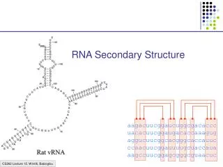
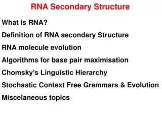
RNA Secondary Structure. aagacuucggaucuggcgacaccc uacacuucggaugacaccaaagug aggucuucggcacgggcaccauuc ccaacuucggauuuugcuaccaua aagccuucggagcgggcguaacuc. Stochastic Context Free Grammars. In an analogy to HMMs, we can assign probabilities to transitions: Given grammar

E N D
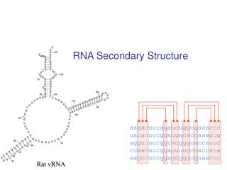
RNA Secondary Structure aagacuucggaucuggcgacaccc uacacuucggaugacaccaaagug aggucuucggcacgggcaccauuc ccaacuucggauuuugcuaccaua aagccuucggagcgggcguaacuc
Stochastic Context Free Grammars In an analogy to HMMs, we can assign probabilities to transitions: Given grammar X1 s11 | … | sin … Xm sm1 | … | smn Can assign probability to each rule, s.t. P(Xi si1) + … + P(Xi sin) = 1
V X Y j i The CYK algorithm (Cocke-Younger-Kasami) Initialization: For i = 1 to N, any nonterminal V, (i, i, V) = log P(V xi) Iteration: For i = 1 to N – 1 For j = i+1 to N For any nonterminal V, (i, j, V) = maxXmaxYmaxik<j (i,k,X) + (k+1,j,Y) + log P(VXY) Termination: log P(x | , *) = (1, N, S) Where * is the optimal parse tree (if traced back appropriately from above)
Evaluation Recall HMMs: Forward: fl(i) = P(x1…xi, i = l) Backward: bk(i) = P(xi+1…xN | i = k) Then, P(x) = k fk(N) ak0 = k a0k ek(x1) bk(1) Analogue in SCFGs: Inside: a(i, j, V) = P(xi…xj is generated by nonterminal V) Outside: b(i, j, V) = P(x, excluding xi…xj is generated by S and the excluded part is rooted at V)
The Inside Algorithm To compute a(i, j, V) = P(xi…xj, produced by V) a(i, j, v) = X Y k a(i, k, X) a(k+1, j, Y) P(V XY) V X Y j i k k+1
Algorithm: Inside Initialization: For i = 1 to N, V a nonterminal, a(i, i, V) = P(V xi) Iteration: For i = 1 to N – 1 For j = i + 1 to N For V a nonterminal a(i, j, V) = X Y k a(i, k, X) a(k+1, j, X) P(V XY) Termination: P(x | ) = a(1, N, S)
The Outside Algorithm b(i, j, V) = Prob(x1…xi-1, xj+1…xN, where the “gap” is rooted at V) Given that V is the right-hand-side nonterminal of a production, b(i, j, V) = X Y k<i a(k, i – 1, X) b(k, j, Y) P(Y XV) Y V X j i k
Algorithm: Outside Initialization: b(1, N, S) = 1 For any other V, b(1, N, V) = 0 Iteration: For i = 1 to N – 1 For j = N down to i For V a nonterminal b(i, j, V) = X Y k<i a(k, i – 1, X) b(k, j, Y) P(Y XV) + X Y k<i a(j + 1, k, X) b(i, k, Y) P(Y VX) Termination: It is true for any i, that: P(x | ) = X b(i, i, X) P(X xi)
Learning for SCFGs We can now estimate c(V) = expected number of times V is used in the parse of x1….xN 1 c(V) = –––––––– 1iNijN a(i, j, V) b(i, j, V) P(x | ) 1 c(VXY) = –––––––– 1iNi<jN ik<j b(i, j, V) a(i, k, X) a(k+1, j, Y) P(VXY) P(x | )
Learning for SCFGs Then, we can re-estimate the parameters with EM, by: c(VXY) Pnew(VXY) = –––––––––––– c(V) c(V a) i: xi = a b(i, i, V) P(V a) Pnew(V a) = –––––––––– = –––––––––––––––––––––––––––––––– c(V) 1iNi<jN a(i, j, V) b(i, j, V)
Summary: SCFG and HMM algorithms GOALHMM algorithm SCFG algorithm Optimal parse Viterbi CYK Estimation Forward Inside Backward Outside Learning EM: Fw/Bck EM: Ins/Outs Memory Complexity O(N K) O(N2 K) Time Complexity O(N K2) O(N3 K3) Where K: # of states in the HMM # of nonterminals in the SCFG
position i length l 5’ 5’ position i 3’ 3’ position j position j The Zuker algorithm – main ideas Models energy of a fold in terms of specific features: • Pairs of base pairs (stacked pairs) • Bulges • Loops (size, composition) • Interactions between stem and loop position j’ positions i 5’ position j 3’
Comparison of SCFGs and Physics Models physics-based models stochastic context-free grammars P(x, y) ∆E(x, y) Find highest scoring pseudoknot-free structure via dynamic programming.
ΔEUA/AU Comparison of SCFGs and Physics Models PHYSICS-BASED MODELS SCFGS • parameters measured manually • necessarily general-purpose • energetics determines structure • most accurate in practice • train parameters automatically • easily tuned to specific data • grammar rules arbitrary • less accurate in practice Can we get the accuracy of physics-based methods and the parameter learning ease of probabilistic methods?
Physics-based models Conditional log-linear models (CLLMs) -- CONTRAfold In energy-based models, the free energy of a structure y is a linear function of features: In CONTRAfold, the logarithm of the probability of a structure y is a linear function of features: “score” of structure y features parameters where
Conditional log-linear models (CLLMs) -- CONTRAfold In CONTRAfold, the logarithm of the probability of a structure y is a linear function of features: “score” of structure y features parameters Key points: (1) We can define set of features that we suspect to be energetically important (2) Parameters w learned automatically and “useless” features are discarded (2) Model is extensible
A G C A G A G U G G … Posterior Decoding for Structure Prediction • Compute a base-pairing probability matrix for sequence x • Find secondary structure maximizing E[correct pairings] + E[correct unpaired bases] … = 1 A G C A G A G U G G = 8 = 1024
Modeling multiple sequences aligned sequences x1,…,xn Given: Compute sequence weights based on evolutionary tree… …then modify scoring function appropriately. 6 5 4 1 3 2
Evaluation Methodology 5s rRNA Example #1 GcvB RNA Fold A Example #2 U14 snoRNA rfam … RNase P … Fold B Example #151 tmRNA 151 independent examples Two-fold cross validation 503 annotated families
Comparison of methods for RNA structure prediction 0.8 CONTRAfold (multi) CONTRAfold (single) 0.7 Alifold (multi) CONTRAfold (single) 0.6 Mfold Pfold (multi) RNAfold (single) Sensitivity 0.5 CONTRAfold (single) Pfold (single) 0.4 0.3 0.4 0.5 0.6 0.7 0.8 0.9 Specificity
Probabilistic Models for Biosequences DNA Sequence, Parse: atcgacggcggctacgtatctcagcagctgctgtgtagtgctgtcgctgtgctgtgtcgagctgagagagagagcgtcgtagctcgatcactgtggatggctgatatagctacgagcgcggcgctatgtctatgtgttgctatg exon, intron, intergenic HMM EXON EXON EXON EXON EXON INTRON INTRON INTRON INTRON Prob-CFG Sequence, Parse: agucuucacugaaugugauggacacuccgagacu ((((..(((.....))).((((...)))).)))) Hairpin, Loop, Stem, … ---Q--------FKAGYCDEPADEG ALGQDMVTVAWCFKAGYCDEPAFEG AELTMPG--M-MTFVMEIKVT--HP AELTMPGNMMNMTFV---KVTDMHP GN----FH-WTWQ--LY--LLPCKD GNTPKDFHDWT-QLVLYTRVLPPKD Sequence, Sequence, Parse: AELTMPG--M-MTFVMEIKVT--HPGN----FH-WTWQ--LYTRLL AELTMPGNMMNMTFV---KVTDMHPGNTPKDFHDWT-QLVLY--VL MMMMMMMXXMXMMMMYYYMMMXXMMMMXXXXMMXMMYMXXMMYYMM Match, GapX, GapY Pair-HMM
Motifs are preferentially conserved across evolution Gal4 TBP GAL4 GAL4 GAL4 GAL4 MIG1 MIG1 TBP Factor footprint Conservation island Gal10 Gal1 GAL10 Scer TTATATTGAATTTTCAAAAATTCTTACTTTTTTTTTGGATGGACGCAAAGAAGTTTAATAATCATATTACATGGCATTACCACCATATACA Spar CTATGTTGATCTTTTCAGAATTTTT-CACTATATTAAGATGGGTGCAAAGAAGTGTGATTATTATATTACATCGCTTTCCTATCATACACA Smik GTATATTGAATTTTTCAGTTTTTTTTCACTATCTTCAAGGTTATGTAAAAAA-TGTCAAGATAATATTACATTTCGTTACTATCATACACA Sbay TTTTTTTGATTTCTTTAGTTTTCTTTCTTTAACTTCAAAATTATAAAAGAAAGTGTAGTCACATCATGCTATCT-GTCACTATCACATATA * * **** * * * ** ** * * ** ** ** * * * ** ** * * * ** * * * Scer TATCCATATCTAATCTTACTTATATGTTGT-GGAAAT-GTAAAGAGCCCCATTATCTTAGCCTAAAAAAACC--TTCTCTTTGGAACTTTCAGTAATACG Spar TATCCATATCTAGTCTTACTTATATGTTGT-GAGAGT-GTTGATAACCCCAGTATCTTAACCCAAGAAAGCC--TT-TCTATGAAACTTGAACTG-TACG Smik TACCGATGTCTAGTCTTACTTATATGTTAC-GGGAATTGTTGGTAATCCCAGTCTCCCAGATCAAAAAAGGT--CTTTCTATGGAGCTTTG-CTA-TATG Sbay TAGATATTTCTGATCTTTCTTATATATTATAGAGAGATGCCAATAAACGTGCTACCTCGAACAAAAGAAGGGGATTTTCTGTAGGGCTTTCCCTATTTTG ** ** *** **** ******* ** * * * * * * * ** ** * *** * *** * * * Scer CTTAACTGCTCATTGC-----TATATTGAAGTACGGATTAGAAGCCGCCGAGCGGGCGACAGCCCTCCGACGGAAGACTCTCCTCCGTGCGTCCTCGTCT Spar CTAAACTGCTCATTGC-----AATATTGAAGTACGGATCAGAAGCCGCCGAGCGGACGACAGCCCTCCGACGGAATATTCCCCTCCGTGCGTCGCCGTCT Smik TTTAGCTGTTCAAG--------ATATTGAAATACGGATGAGAAGCCGCCGAACGGACGACAATTCCCCGACGGAACATTCTCCTCCGCGCGGCGTCCTCT Sbay TCTTATTGTCCATTACTTCGCAATGTTGAAATACGGATCAGAAGCTGCCGACCGGATGACAGTACTCCGGCGGAAAACTGTCCTCCGTGCGAAGTCGTCT ** ** ** ***** ******* ****** ***** *** **** * *** ***** * * ****** *** * *** Scer TCACCGG-TCGCGTTCCTGAAACGCAGATGTGCCTCGCGCCGCACTGCTCCGAACAATAAAGATTCTACAA-----TACTAGCTTTT--ATGGTTATGAA Spar TCGTCGGGTTGTGTCCCTTAA-CATCGATGTACCTCGCGCCGCCCTGCTCCGAACAATAAGGATTCTACAAGAAA-TACTTGTTTTTTTATGGTTATGAC Smik ACGTTGG-TCGCGTCCCTGAA-CATAGGTACGGCTCGCACCACCGTGGTCCGAACTATAATACTGGCATAAAGAGGTACTAATTTCT--ACGGTGATGCC Sbay GTG-CGGATCACGTCCCTGAT-TACTGAAGCGTCTCGCCCCGCCATACCCCGAACAATGCAAATGCAAGAACAAA-TGCCTGTAGTG--GCAGTTATGGT ** * ** *** * * ***** ** * * ****** ** * * ** * * ** *** Scer GAGGA-AAAATTGGCAGTAA----CCTGGCCCCACAAACCTT-CAAATTAACGAATCAAATTAACAACCATA-GGATGATAATGCGA------TTAG--T Spar AGGAACAAAATAAGCAGCCC----ACTGACCCCATATACCTTTCAAACTATTGAATCAAATTGGCCAGCATA-TGGTAATAGTACAG------TTAG--G Smik CAACGCAAAATAAACAGTCC----CCCGGCCCCACATACCTT-CAAATCGATGCGTAAAACTGGCTAGCATA-GAATTTTGGTAGCAA-AATATTAG--G Sbay GAACGTGAAATGACAATTCCTTGCCCCT-CCCCAATATACTTTGTTCCGTGTACAGCACACTGGATAGAACAATGATGGGGTTGCGGTCAAGCCTACTCG **** * * ***** *** * * * * * * * * ** Scer TTTTTAGCCTTATTTCTGGGGTAATTAATCAGCGAAGCG--ATGATTTTT-GATCTATTAACAGATATATAAATGGAAAAGCTGCATAACCAC-----TT Spar GTTTT--TCTTATTCCTGAGACAATTCATCCGCAAAAAATAATGGTTTTT-GGTCTATTAGCAAACATATAAATGCAAAAGTTGCATAGCCAC-----TT Smik TTCTCA--CCTTTCTCTGTGATAATTCATCACCGAAATG--ATGGTTTA--GGACTATTAGCAAACATATAAATGCAAAAGTCGCAGAGATCA-----AT Sbay TTTTCCGTTTTACTTCTGTAGTGGCTCAT--GCAGAAAGTAATGGTTTTCTGTTCCTTTTGCAAACATATAAATATGAAAGTAAGATCGCCTCAATTGTA * * * *** * ** * * *** *** * * ** ** * ******** **** * Scer TAACTAATACTTTCAACATTTTCAGT--TTGTATTACTT-CTTATTCAAAT----GTCATAAAAGTATCAACA-AAAAATTGTTAATATACCTCTATACT Spar TAAATAC-ATTTGCTCCTCCAAGATT--TTTAATTTCGT-TTTGTTTTATT----GTCATGGAAATATTAACA-ACAAGTAGTTAATATACATCTATACT Smik TCATTCC-ATTCGAACCTTTGAGACTAATTATATTTAGTACTAGTTTTCTTTGGAGTTATAGAAATACCAAAA-AAAAATAGTCAGTATCTATACATACA Sbay TAGTTTTTCTTTATTCCGTTTGTACTTCTTAGATTTGTTATTTCCGGTTTTACTTTGTCTCCAATTATCAAAACATCAATAACAAGTATTCAACATTTGT * * * * * * ** *** * * * * ** ** ** * * * * * *** * Scer TTAA-CGTCAAGGA---GAAAAAACTATA Spar TTAT-CGTCAAGGAAA-GAACAAACTATA Smik TCGTTCATCAAGAA----AAAAAACTA.. Sbay TTATCCCAAAAAAACAACAACAACATATA * * ** * ** ** ** Is this enough to discover motifs? No. GAL1 slide credits: M. Kellis
Erra Erra Erra Dog Mouse Rat Conservation rate: 37% Known motifs are frequently conserved Human • Across the human promoter regions, the Erra motif: • appears 434 times • is conserved 162 times • Compare to random control motifs • Conservation rate of control motifs: 6.8% • Erra enrichment: 5.4-fold • Erra p-value < 10-50 (25 standard deviations under binomial) Motif Conservation Score (MCS) slide credits: M. Kellis
Finding conserved motifs in whole genomes • Define seed “mini-motifs” • Filter and isolate mini-motifs that are more conserved than average • Extend mini-motifs to full motifs • Validate against known databases of motifs & annotations • Report novel motifs N T C A A C G slide credits: M. Kellis
CGG-11-CCG Test 1: Intergenic conservation Conserved count Total count slide credits: M. Kellis
CGG-11-CCG Higher Conservation in Genes Test 2: Intergenic vs. Coding Intergenic Conservation Coding Conservation slide credits: M. Kellis
CGG-11-CCG Downstream motifs? Most Patterns Test 3: Upstream vs. Downstream Upstream Conservation Downstream Conservation slide credits: M. Kellis
5 6 Y R T C G C A C G A Extend Extend Extend Collapse Extend G T C A C A C G A A T C R Y A C G A Collapse Collapse Collapse R T C G C A C G A Merge 72 Full motifs Full Motifs Constructing full motifs Test 1 Test 2 Test 3 2,000 Mini-motifs R T C A A C G R slide credits: M. Kellis
New New New New New Summary for promoter motifs • 174 promoter motifs • 70 match known TF motifs • 115 expression enrichment • 60 show positional bias 75% have evidence • Control sequences < 2% match known TF motifs < 5% expression enrichment < 3% show positional bias < 7% false positives Most discovered motifs are likely to be functional slide credits: M. Kellis