Download
1 / 88
890 likes | 1.1k Vues
Gene Expression and DNA Chips. Based on slides by Ron Shamir. http://www.bio.davidson.edu/courses/genomics/chip/chip.html. Monitoring Gene Expression. Goal : Simultaneous measurement of expression levels of all genes in one experiment. 2 fundamental biological assumptions:

E N D
Gene Expression and DNA Chips Based on slides by Ron Shamir http://www.bio.davidson.edu/courses/genomics/chip/chip.html
Monitoring Gene Expression • Goal: Simultaneous measurement of expression levels of all genes in one experiment. • 2 fundamental biological assumptions: • Transcription level indicates genes’ regulation. • Only genes that contribute to organism fitness are expressed. => Detecting changes in a gene’s expression level provides clues on the function of its product
Factors controlling expression Post-translational modifications Alternative splicing RNA interference / degradation Chromatin remodeling Pre-mRNA Mature mRNA DNA protein transcription splicing translation
TGAGGC | | | | | | ACTCCG Hybridization • DNA double strands form by “gluing” of complementary single strands • Complementarity rule: A-T, G-C Use probe to identify if target contains a particular sequence
DNA chips / Microarrays • Perform thousands of hybridizations in a single experiment • Variants: • Oligonucleotide arrays • cDNA microarrays • Another distinction • Single channel • Dual channel • Allow global view of cellular processes: Monitor transcription levels of numerous/all genes simultaneously.
A single feature on the chip http://www.affymetrix.com/corporate/media/image_library/
For Flash animation of the technology, see http://www.bio.davidson.edu/Courses/genomics/chip/chip.html
Affymetrix oligo arrays vs cDNA microarrays • Short oligos • Low specificity • High density • Many probes per gene • Synthetic oligos • Absolute exp values • Yield problems • “turnkey” solutions • Price: +++ • Long oligos • High specificity • Lower density • One probe per gene • Probes: cDNAs • Relative exp values • Spotting problems • Custom solutions • Price : ++
… and other technologies • Agilent: • In situ synthesized arrays using ink-jet technology • 60-mer arrays: more specific than Affy’s • Allows custom design without expensive masks • Differential measurements: target vs reference • Nimblegen • Illumina
Comparative genomic hybridization (CGH) microarrays Cells of Interest Known DNA sequences Isolate genomicDNA Glass slide Reference sample Flourescently labeled (almost identical to gene expression arrays, but genomic DNA is hybridized instead of mRNA)
Chromosomes with varying copy number fluctuations from analysis of the tumor cell line SK-BR-3 as compared with the normal reference Robert Lucito et al. Genome Res. 2003; 13: 2291-2305
Single nucleotide polymorphism (SNP) detection SNP: single base sequence variation A/G Target sequence: GCCATGCANGAGTTACTACAGTAGC CGGTACGTTCTCAATGATGTCATCG PM + 4 Allele A MM +4 Allele A CGGTACGTTCTCTATGATGTCATCG CGGTACGTCCTCAATGATGTCATCG PM +4 Allele B CGGTACGTCCTCTATGATGTCATCG MM + 4 Allele B (Affymetrix Human Mapping 500K Array)
Remember Gene Transcription? Transcription Factors (proteins) RNA polymerase (protein) C T A A T G T . . . 5’ 3’ 3’ 5’ G A T T A C A . . . Transcription factors recognize transcription factor binding sites and bind to them, forming a complex. RNA polymerase binds the complex. (eukaryotes)
Using microarrays to measure protein-DNA interactions ChIP-chip: Chromatin immunoprecipitation chip (microarray) (antibodies bind transcription factor of interest) (TF-bound sequences hybridized to microarray) Simon et al., Cell 2001
Mapping transcription factor binding sites in yeast with ChIP-chip Harbison C., Gordon B., et al. Nature 2004
Dynamic role of transcription factors Harbison C., Gordon B., et al. Nature 2004
yfg1D yfg2D yfg3D Other microarray applications:Competitive growth assays Barcode CTAACTC TCGCGCA TCATAAT … Deletion Strain: Growth 6hrs in minimal media Rich media Harvest and label genomic DNA
Measuring relative fitness with a barcode microarray Oligo barcodes matching each strain are also spotted on a DNA microarray
Protein Microarrays • Protein microarrays are lagging behind DNA microarrays • Same idea but immobilized elements are proteins instead of nucleic acids • Number of elements (proteins) on current protein microarrays are limited (approx. 500) • Antibodies for high density microarrays have limitations (cross-reactivities) • Aptamers or engineered antibodies/proteins may be viable alternatives (Aptamers:RNAs that bind proteins with high specificity and affinity)
Applications Screening for: • Small molecule targets • Post-translational modifications • Protein-protein interactions • Protein-DNA interactions • Enzyme assays • Epitope mapping
Label all Proteins in Mixture High-throughput proteomic analysis Haab et al. Genome Biology 2000;1:1-22
MIX IL-1 IL-6 IL-10 VEGF marker protein cytokine Cytokine Specific Microarray (Microarray version of ELISA) Detection system BIOTINYLATED MAb ANTIGEN CAPTURE MAb
Tissue Microarrays • Printing on a slide tiny amounts of tissue • Array many patients in one slide (e.g. 500) • Process all at once (e.g. immunohistochemistry) • Works with archival tissue (paraffin blocks)
Tissue Microarray Alizadeh et al. J Pathol 2001;195:41-52
Normalization is important!! How Gene Expression Data Looks • Entries of the Raw Data matrix: • Ratio values • Absolute values • Distributions… • Row = gene’s expression pattern / • fingerprint vector • Column = experiment/condition’s • profile conditions Expression levels, “Raw Data” genes
From the Raw Data matrix we compute the similarity matrix S. Sij reflects the similarity of the expression patterns of gene i and gene j. Data Preprocessing conditions Expression levels, “Raw Data” genes • Input: Real-valued raw data matrix. • Compute the similarity matrix (dot product/correlation/…)
DNA chips: Applications • Deducing functions of unknown genes • (similar expression pattern similar function) • Identifying disease profiles • Deciphering regulatory mechanisms • (co-expression co-regulation). • Classification of biological conditions • Genotyping • Drug development • … Analysis requires clustering of genes/conditions.
Pearson Correlation Coefficient, r. Values are in [-1,1] interval • Gene expression over d experiments is a vector in Rd, e.g. for gene C: (0, 3, 3.58, 4, 3.58, 3) • Given two vectors X and Y that contain N elements, we calculate r as follows: Cho & Won, 2003
Intuition for Pearson Correlation Coefficient r(v1,v2) close to 1: v1, v2 highly correlated. r(v1,v2) close to -1: v1, v2 anti correlated. r(v1,v2) close to 0: v1, v2 not correlated.
Pearson Correlation and p-Values When entries in v1,v2 are distributed according to normal distribution, can assign (and efficiently compute) p-Values for a given result. These p-Values are determined by the Pearson correlation coefficient, r, and the dimension, d, of the vectors. For same r, vectors of higher dimension will be assigned more significant (smaller) p-Value.
Spearman Rank Order Coefficient(a close relative of Pearson, non parametric) • Replace each entry xi by its rank in vector x. • Then compute Pearson correlation coefficients of rank vectors. • Example: X = Gene C = (0, 3.00, 3.41, 4, 3.58, 3.01) Y = Gene D = (0, 1.51, 2.00, 2.32, 1.58, 1) • Ranks(X)= (1,2,4,6,5,3) • Ranks(Y)= (1,3,5,6,4,2) • Ties should be taken care of, but: (1) rare (2) can randomize (small effect)
From Pearson Correlation Coefficients to a Gene Network • Compute correlation coefficient for all pairs of genes (what about missing data?) • Choose p-Value threshold. • Put an edge between gene i and gene j iff p-Value exceeds threshold.
Clustering: Objective • Group elements (genes) to clusters satisfying: • Homogeneity: Elements inside a cluster are highly similar to each other. • Separation: Elements from different clusters have low similarity to each other.
An Alternative View • Form a tree-hierarchy of the input elements satisfying: • More similar elements are placed closer along the tree. • Or: Tree distances reflect element similarity • Note: No explicit partition into clusters.
Hierarchical Representations (2) Dendrogram: rooted tree, usually binary, and all root-leaf distances are equal 5.0 4.5 2.8 1 2 3 4 1 2 3 4
Neighbor Joining Algorithm Saitou & Nei, 87 • Input: Distance matrix Dij; Initially eachelement is a cluster. • Find min element Drs in D; merge clusters r,s • Delete elts. r,s, add new elt. t with Dit=Dti=(Dir+ Dis – Drs)/2 • Repeat • Present the hierarchy as a tree with similar elements near each other
Hierarchical Clustering: Average LinkageSokal & Michener 58, Lance & Williams 67 • Input: Distance matrix Dij; Initially eachelement is a cluster. nr- size of cluster r • Find min element Drs in D; merge clusters r,s • Delete elts. r,s, add new elt. t with Dit=Dti=nr/(nr+ns)•Dir+ ns/(nr+ns) •Dis • Repeat
A General FrameworkLance & Williams 67 • Input: Distance matrix Dij; Initially eachelement is a cluster. • Find min element Drs in D, merge clusters r,s • Delete elts. r,s, add new elt. t with Dit=Dti=rDir+ sDis + |Dir-Dis|