Download
1 / 43
520 likes | 1.32k Vues
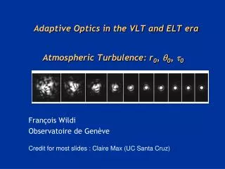
Adaptive Optics in the VLT and ELT era. Atmospheric Turbulence: r 0 , 0 , 0. François Wildi Observatoire de Genève Credit for most slides : Claire Max (UC Santa Cruz). r 0 sets the number of degrees of freedom of an AO system.

E N D
Adaptive Optics in the VLT and ELT era Atmospheric Turbulence: r0, 0,0 François Wildi Observatoire de Genève Credit for most slides : Claire Max (UC Santa Cruz)
r0 sets the number of degrees of freedom of an AO system • Divide primary mirror into “subapertures” of diameter r0 • Number of subapertures ~ (D / r0)2where r0 is evaluated at the desired observing wavelength • Example: Keck telescope, D=10m, r0 ~ 60 cm at l = 2mm. (D / r0)2 ~ 280. Actual # for Keck : ~250.
About r0 • Define r0 as telescope diameter where optical transfer functions of the telescope and atmosphere are equal • r0 is separation on the telescope primary mirror where phase correlation has fallen by 1/e • (D/r0)2is approximate number of speckles in short-exposure image of a point source • D/r0 sets the required number of degrees of freedom of an AO system • Timescales of turbulence • Isoplanatic angle: AO performance degrades as astronomical targets get farther from guide star
What about temporal behavior of turbulence? • Questions: • What determines typical timescale without AO? • With AO?
A simplifying hypothesis about time behavior • Almost all work in this field uses “Taylor’s Frozen Flow Hypothesis” • Entire spatial pattern of a random turbulent field is transported along with the wind velocity • Turbulent eddies do not change significantly as they are carried across the telescope by the wind • True if typical velocities within the turbulence are small compared with the overall fluid (wind) velocity • Allows you to infer time behavior from measured spatial behavior and wind speed:
Cartoon of Taylor Frozen Flow • From Tokovinin tutorial at CTIO: • http://www.ctio.noao.edu/~atokovin/tutorial/
Order of magnitude estimate • Time for wind to carry frozen turbulence over a subaperture of size r0 (Taylor’s frozen flow hypothesis): t0 ~ r0 / V • Typical values: • l = 0.5 mm, r0 = 10 cm, V = 20 m/sec t0 = 5 msec • l = 2.0 mm, r0 = 53 cm, V = 20 m/sec t0 = 265 msec • l = 10 mm, r0 = 36 m, V = 20 m/sec t0 = 1.8 sec • Determines how fast an AO system has to run
But what wind speed should we use? • If there are layers of turbulence, each layer can move with a different wind speed in a different direction! • And each layer has different CN2 V1 Concept Question: What would be a plausible way to weight the velocities in the different layers? V2 V3 V4 ground
Rigorous expressions for t0 take into account different layers • fG Greenwood frequency 1 / t0 • What counts most are high velocities V where CN2 is big Hardy§9.4.3
Short exposures: speckle imaging • A speckle structure appears when the exposure is shorter than the atmospheric coherence time 0 • Time for wind to carry frozen turbulence over a subaperture of size r0
Structure of an AO image • Take atmospheric wavefront • Subtract the least square wavefront that the mirror can take • Add tracking error • Add static errors • Add viewing angle • Add noise
atmospheric turbulence + AO • AO will remove low frequencies in the wavefront error up to f=D 2/n, where n is the number of actuators accross the pupil • By Fraunhoffer diffraction this will produce a center diffraction limited core and halo starting beyond 2D/n PSD(f) 2D/n f
atmospheric turbulence + AO II Spatially Filtered SH Optimization of the spatial filter size Study of BB impact NB filters for optimal results BB [0.5 – 0.9]m : perf acceptable => OK for “faint” GS (mag 9) WCOG : confirmation of the gain in perf (simul AND experimentation) (see Pres. T. Fusco) WFS band : 0.5-0.9 0.7-0.9 monochromatic
Detectivity curves • Detectivity at 5: evaluated by variance computation in the object estimation maps for 100 samples of both aberrations and noise Single difference Single image Double difference Our approach The proposed approach performs better than the alternatives: Detectivity increased by a factor ~10 over the whole field Estimated gain in magnitude difference ~ 2.5 Limited by static speckle Limited by noise
Anisoplanatism: how does AO image degrade as you move farther from guide star? • Composite J, H, K band image, 30 second exposure in each band • Field of view is 40”x40” (at 0.04 arc sec/pixel) • On-axis K-band Strehl ~ 40%, falling to 25% at field corner credit: R. Dekany, Caltech
More about anisoplanatism: AO image of sun in visible light 11 second exposure Fair Seeing Poor high altitude conditions From T. Rimmele
AO image of sun in visible light: 11 second exposure Good seeing Good high altitude conditions From T. Rimmele
What determines how close the reference star has to be? Reference Star Science Object Turbulence z Common Atmospheric Path Telescope Turbulence has to be similar on path to reference star and to science object Common path has to be large Anisoplanatism sets a limit to distance of reference star from the science object
Expression for isoplanatic angle 0 • Strehl = 0.38 at = 0 0is isoplanatic angle 0is weighted by high-altitude turbulence (z5/3) • If turbulence is only at low altitude, overlap is very high. • If there is strong turbulence at high altitude, not much is in common path Common Path Telescope
Isoplanatic angle, continued • Isoplanatic angle 0 is weighted by z5/3 CN2(z) • Simpler way to remember 0 Hardy§3.7.2
Review • r0 (“Fried parameter”) • Sets number of degrees of freedom of AO system • 0 (or Greenwood Frequency ~ 1 / 0 ) t0 ~ r0 / V where • Sets timescale needed for AO correction • 0 (or isoplanatic angle) • Angle for which AO correction applies
Part 2: • What determines the total wavefront error for an AO system
How to characterize a wavefront that has been distorted by turbulence • Path length difference Dz where kDz is the phase change due to turbulence • Variance s2 = <(k Dz)2 > • If several different effects cause changes in the phase, stot2 = k2 <(Dz1 + Dz2 + ....)2 > = k2 <(Dz1)2 + ( Dz2 )2 ...) > stot2 = s12 + s22 + s32 + ... radians2 or (Dz)2 = (Dz1)2 + (Dz2)2 + (Dz3)2 + ..... nm2
Question • List as many physical effects as you can that might contribute to overall wavefront error stot2 Total wavefront error stot2 = s12 + s22 + s32 + ...
Elements of an adaptive optics system DM fitting error Not shown: tip-tilt error, anisoplanatism error Non-common path errors Phase lag, noise propagation Measurement error
Hardy Figure 2.32
Wavefront errors due to 0 , 0 • Wavefront phase variance due to t0 = fG-1 • If an AO system corrects turbulence “perfectly” but with a phase lag characterized by a time t, then • Wavefront phase variance due to 0 • If an AO system corrects turbulence “perfectly” but using a guide star an angle away from the science target, then Hardy Eqn 9.57 Hardy Eqn 3.104
Deformable mirror fitting error • Accuracy with which a deformable mirror with subaperture diameter d can remove aberrations sfitting2= m ( d / r0 )5/3 • Constant m depends on specific design of deformable mirror • For segmented mirror that corrects tip, tilt, and piston (3 degrees of freedom per segment) m = 0.14 • For deformable mirror with continuous face-sheet, m = 0.28
Image motion or “tip-tilt” also contributes to total wavefront error image motion in radians is indep of l • Turbulence both blurs an image and makes it move around on the sky (image motion). • Due to overall “wavefront tilt” component of the turbulence across the telescope aperture • Can “correct” this image motion either by taking a very short time-exposure, or by using a tip-tilt mirror (driven by signals from an image motion sensor) to compensate for image motion (Hardy Eqn 3.59 - one axis)
Scaling of tip-tilt with l and D: the good news and the bad news • In absolute terms, rms image motion in radians is independent of l, anddecreases slowly as D increases: • But you might want to compare image motion to diffraction limit at your wavelength: Now image motion relative to diffraction limit is almost ~ D, and becomes larger fraction of diffraction limit for small l
Long exposures, no AO correction • “Seeing limited”: Units are radians • Seeing disk gets slightly smaller at longer wavelengths: FWHM ~ / -6/5 ~ -1/5 • For completely uncompensated images, wavefront error • s2uncomp = 1.02 ( D / r0 )5/3
Scaling of tip-tilt for uncompensated or “seeing limited” images • Image motion is larger fraction of “seeing disk” at longer wavelengths
Correcting tip-tilt has relatively large effect, for seeing-limited images • For completely uncompensated images s2uncomp = 1.02 ( D / r0 )5/3 • If image motion (tip-tilt) has been completely removed • s2tiltcomp = 0.134 ( D / r0 )5/3 • (Tyson, Principles of AO, eqns 2.61 and 2.62) • Removing image motion can (in principle) improve the wavefront variance of an uncompensated image by a factor of 10 • Origin of statement that “Tip-tilt is the single largest contributor to wavefront error”
But you have to be careful if you want to apply this statement to AO correction • If tip-tilt has been completely removed s2tiltcomp = 0.134 ( D / r0 )5/3 • But typical values of ( D / r0 ) are10-50 in near-IR • VLT, D=8 m, r0 = 50 cm, ( D/r0 ) = 17 s2tiltcomp = 0.134 ( 17 )5/3 ~ 15 so wavefront phase variance is >> 1 • Conclusion: if( D/r0 ) >> 1, removing tilt alone won’t give you anywhere near a diffraction limited image
Effects of turbulence depend on size of telescope • Coherence length of turbulence: r0 (Fried’s parameter) • For telescope diameter D (2 - 3) x r0 : Dominant effect is "image wander" • As D becomes >> r0 : Many small "speckles" develop • Computer simulations by Nick Kaiser: image of a star, r0 = 40 cm D = 2 m D = 8 m D = 1 m
Effect of atmosphere on long and short exposure images of a star Correcting tip-tilt only is optimum for D/r0 ~ 1 - 3 Hardy p. 94 Vertical axis is image size in units of l/r0 Image motion only FWHM = l/D
Error budget concept (sum of s2 ’s) stot2 = s12 + s22 + s32+ ... • There’s not much gained by making any particular term much smaller than all the others: try to equalize • Individual terms we know so far: • Anisoplanatism sanisop2 = ( / 0 )5/3 • Temporal error stemporal2 = 28.4 (t / t0 )5/3 • Fitting error sfitting2 = m ( d / r0 )5/3 • Need to find out: • Measurement error (wavefront sensor) • Non-common-path errors (calibration) • .......
Error budget so far stot2 = sfitting2 + sanisop2 + stemporal2+ smeas2 + scalib2 √ √ √ Still need to work on these two
We want to relate phase variance to the “Strehl ratio” • Two definitions of Strehl ratio (equivalent): • Ratio of the maximum intensity of a point spread function to what the maximum would be without aberrations • The “normalized volume” under the optical transfer function of an aberrated optical system
Examples of PSF’s and their Optical Transfer Functions Seeing limited OTF Seeing limited PSF 1 Intensity -1 l / D l / r0 r0 / l D / l Diffraction limited PSF Diffraction limited OTF 1 Intensity -1 l / r0 l / D D / l r0 / l
Relation between variance and Strehl • “Maréchal Approximation” • Strehl ~ exp(- s2) where s2is the total wavefront variance • Valid when Strehl > 10% or so • Under-estimate of Strehl for larger values of s2
Relation between Strehl and residual wavefront variance Strehl ~ exp(-s2) Dashed lines: Strehl ~ (r0/D)2 for high wavefront variance
Error Budgets: Summary • Individual contributors to “error budget” (total mean square phase error): • Anisoplanatism sanisop2 = ( / 0 )5/3 • Temporal errorstemporal2 = 28.4 (t / t0 )5/3 • Fitting errorsfitting2 = m ( d / r0 )5/3 • Measurement error • Calibration error, ..... • In a different category: • Image motion <a2>1/2 = 2.56 (D/r0)5/6 (l/D) radians2 • Try to “balance” error terms: if one is big, no point struggling to make the others tiny
![[0 1 0]](https://cdn0.slideserve.com/536424/slide1-dt.jpg)