Download
1 / 17
170 likes | 331 Vues
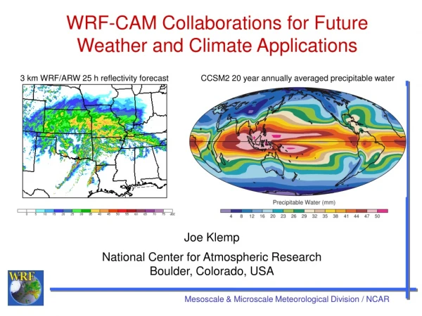
Effects of the Great Salt Lake’s Temperature and Size on the Regional Precipitation in the WRF Model. Joe Grim Jason Knievel National Center for Atmospheric Research Research Applications Laboratory ATEC Project Erik Crosman University of Utah. Introduction.

E N D
Effects of the Great Salt Lake’s Temperature and Size on the Regional Precipitation in the WRF Model Joe Grim Jason Knievel National Center for Atmospheric Research Research Applications Laboratory ATEC Project Erik Crosman University of Utah
Introduction • Great Salt Lake is largest endorheic lake in Western Hemisphere • Size varied 71% (2,460-8,500 km2) during past 50 years • Size, surface temperature and salinity typically not represented well in operational forecast models • Our study • Varies lake size for case study sensitivity comparisons • Calculates MODIS lake surface temperatures similar to Knievel et al. (2010).
WRF Simulations with Varying Lake Size • Model Setup • 4 Domains • 1.1 km for d04 • Same Physics Options as Colorado Headwaters Project • Microphsyics: Thompson 7-Class • RRTM LongwaveRadiation • Dudhia Shortwave Radiation • Monin-Obukhov Surface Layer • Noah Land-Surface • YSU PBL • Two Simulations • Big Lake: 1986 Lake Size: 8500 km2 • Small Lake: 1964 Lake Size: 2460 km2
Observed Salt Lake City Radar Analysis Radar Data Missing During Early Portion of the Period Shortly After Cold Frontal Passage Switching to Wind Parallel Bands Laterwith Wind Shift to NWerly Shore Parallel Band Before Cold Frontal Passage Lake Enhanced Snow
Previous “SST” Results from NASA NYC Project • Operational Real-Time Global (RTG) • Continuous Coverage from Satellite & In-Situ • Coarse Effective Resolution (~100 km) • MODIS 12-day Composite for NASA NYC • Nearly-Continuous Coverage from MODIS Only (holes filled with RTG) • Fine Resolution (~10 km) • Showed greatest skill in shallow near-shore locations
Most of Great Salt Lake is Shallow and Close to Shore • How Do MODIS “SSTs” Perform for GSL? • Most operational models (e.g., NAM) use climatology for GSL temperature • We want to perform a more in-depth analysis to see if we can make an improvement over climatology
NASA SST Product Availability for the Great Salt Lake DAY NIGHT Data void in summer and winter
Must Create Our Own Great Salt Lake Water Temperature Product QCed Land Surface Temperature Plots over GSL for 12 Days Temperature (°C)
Processing Steps • Quality Control from Concurrent Fields • Sky Cover • QC Parameter • 11 µm Emissivity • 12 µm Emissivity • Viewing Angle • Quality Control from Other Satellite Overpasses • Intraday Comparisons (Terra vs. Aqua) • Day-to-Day Temperature Comparisons • Bias Correct from Comparisons with Buoy • Determination of Optimal # of Days for Temporal Composite • Availability % • Minimize Errors vs. Buoy Observations • Fill in Remaining Spatial Gaps with Nearest Neighbor Technique
Fill in Spatial Gaps Using Nearest Valid Pixel 99.7% Availability for 2010-2011 Mean Absolute Difference vs. Buoy: 0.7 °C (1.6 °C for climatology)
Conclusions • Lake Size Can Have Large Effect on Nearby Mesoscale Processes • e.g., Produce Large Precipitation Differences during Lake Effect/Enhanced Events • Temporal and Spatial QCing & Compositing of MODIS Data Produces • Nearly Continuous Water Surface Temperature Fields for Use in Operational Models • Spatial Heterogeniety, unlike using only single buoy reading for entire lake • Accurate LST estimates (MAD = 0.7 °C) • Caveat: Verified against same data set used for calibration • Will test on 2012
Future Work • Perform WRF Simulations Using Climatology vs. MODIS Composite • Implement techniques operationally in WRF for Army Ranges • Real-time lake size • Real-time lake temperatures (currently use climatology) • Vary salinity (and thus water surface heat and moisture exchange) for further sensitivity simulations
References Knievel, Jason C., Daran L. Rife, Joseph A. Grim, Andrea N. Hahmann, Joshua P. Hacker, Ming Ge, Henry H. Fisher, 2010: A simple technique for creating regional composites of sea surface temperature from MODIS for use in operational mesoscaleNWP. J. Appl. Meteor. Climatol., 49, 2267–2284. Crosman, E. T., and J. D. Horel, 2009: MODIS-derived surface temperature of the Great Salt Lake. Remote Sensing of Environment, 113, 73-81.