Physically-Based Simulation on Graphics Hardware
Explore the application of physically-based simulation in games using graphics hardware, covering topics such as rigid body dynamics, water simulation, visual effects, and parallel processing benefits.

Physically-Based Simulation on Graphics Hardware
E N D
Presentation Transcript
Physically-Based Simulation on Graphics Hardware Mark J. Harris UNC Chapel Hill Greg James NVIDIA Corp. Elder Scrolls III: Morrowind
Physically-Based Simulation • Games are using it • Newtonian physics on the CPU • Rigid body dynamics, projectile and particle motion, inverse kinematics • PDEs and non-linear fun on the CPU/VPU • Water simulation (geometry), special effects • It’s cool, but computationally expensive • Complex non-rigid body dynamics & effects • Water, fire, smoke, fluid flow, glow and HDR • High data bandwidth • Lots of math. Much can be done in parallel
Physically-Based Simulation • Graphics processors are perfect for many simulation algorithms • GeForce 3, 4, GeForce FX, Radeon 9xxx • Direct3D8, Direct3D9 support • Free parallelism, GFlops of math, vector processors • 500 Mhz * 8 pix/clk * 4-floats/pixel = 16 GFlops • Current generation has 16 and 32-bit float precision throughout
Games Doing Simulation and Effects on the GPU (partial list) • PC • Elder Scrolls III: Morrowind • Dark Age of Camelot • Tron 2.0 • Tiger Woods 2.0 • 3DMark2003 • XBox • Halo 2 • Wreckless • PS2 • Baldur’s Gate: Dark Alliance
Visual Simulation • Goal is visual interest • Not numerical accuracy • Often not physical accuracy, just the right feel • Approximations and home-brew methods produce great results • Dynamic scenes, interesting reaction to inputs • If the user is convinced, the method, math, and stability don’t matter!! • 8-bit math and results are ok (last year’s hardware) Elder Scrolls III: Morrowind Bethesda Softworks
Practical Techniques • Interesting phenomena • Useful in real-time scenes • Interactive: Can react to characters, events, and the environment • Effects themselves run at 150-500 fps • Doesn’t kill your framerate • Free modular source code • Developer support • Just ask!
How Does It Work? • Graphics processor renders colors • 8 bits per channel or 32 bits per channel • Colors store the state of the simulation • Blue = 1D position, Green = velocity, Red = force • RGB1 = 3D position, RGB2 = 3D velocity • Rendered colors are read back in and used to render new colors (the next time step) • Render To Texture (“RTT”) • Redirect color to a vertex stream (coming soon to OGL) • Iterate, storing temporaries and results in video memory textures
The Result • Graphics hardware textures are used to create or animate other textures • Animated textures can be used in the scene • Data & temporaries might never been seen • Fast, endless, non-repeating or repeating • A little video memory can go a long way! • Much less storage than ‘canned’ animation • 2 textures can make an endless animation RTT DISPLAY RTT
What Can We Do? • Blur and glow • Animated blur, dissolves, distortions • Animated bump maps • Normal maps, EMBM du/dv maps • Cellular Automata (CA) • Noise, animated patterns • Allows for very complex rules • Physical Simulation • On N-dimensional grids • CA, CML, LBM
How to do it • Objective - Keep it ALL on the GPU! • Efficient calculation • No CPU or GPU pipeline stalls for synchronization • No AGP texture transfer between CPU and GPU • Saves a ton of CPU MHz • Geometry drives the processing • Programmable Pixel Shaders do the math • Each Texture Coordinate reads data from specific location • Location is absolute or relative to pixel being rendered • N texture fetches gives N RGBA data inputs • Sample neighboring texels, or any texels • Compute slopes, derivatives, gradients, divergence
Geometry Drives Processing • Textures store input, temporary, and final results • Geometry’s texture coordinates get interpolated • Fetch texture data at interpolated coords • Do calculations on the texture data in the programmable pixel shader
Example 1: Sample and Combine Each Texel’s Neighbors • Source texture ‘src’ is (x,y) texels in size • SetTexture(0, src); • SetTexture(1, src); • SetTexture(2, src); • SetTexture(3, src); • texel width ‘tw’ = 1/x • texel height ‘th’ = 1/y • Render target is also a texture (x,y) pixels in size • SetRenderTarget(dest_tex); C A B D
tc0 = (0,0) Quad tc0 = (1,1) VC VB VA VD Example 1 Contd. • Render a quad exactly covering the render target • Texture coords from (0,0) to (1,1) • Unmodified, these would copy the source exactly into the dest • Vertex Shader reads input coordinate ‘tc0’ • Writes 4 output coordinates • Each coordinate offset by a different vector: VA, VB, VC, VD VA = (-tw, 0, 0, 0) VD = (0, th, 0, 0) out_T0 = tc0 + VA out_T1 = tc0 + VB out_T2 = tc0 + VC out_T3 = tc0 + VD
VC src src src VA src VB Example 1 Contd. • The offset coordinates translate the source textures, so that a pattern of neighbors is sampled for each pixel rendered
Sampling From Neighbors • When destination pixel, is rendered If VA, VB, VC, VD are (0,0) then: • t0 = pixel at (2,1) • t1 = pixel at (2,1) • t2 = pixel at (2,1) • t3 = pixel at (2,1) If VA=(-tw,0), VB=(tw,0), VC=(0,-th) VD=(0,th) then: • t0 = pixel A at (1,1) • t1 = pixel B at (3,1) • t2 = pixel C at (2,0) • t3 = pixel D at (2,2) C A B D 0 1 2 3
C A B D E F 0 1 2 3 Sampling From Neighbors • Same pattern is sampled for each pixel rendered to the destination • When pixel is rendered, it samples from: • t0 = pixel E • t1 = pixel D • t2 = pixel A • t3 = pixel F
Example 2: Samples Processed in Pixel Shader • Do whatever math you like out color = (t0 + t1 + t2 + t3)/4 out color = (t0-t1) CROSS (t2-t3) etc... (t0 + t1 + t2 + t3)/4 src dest
Simple Fire Effect • Blur and scroll upward • Trails of blur emerge from bright source ‘embers’ at the bottom VA VC VB VD
Fire Effect • Jitter texture sampling • Vary VA..VD offsets for a wind effect • Turbulence: Tessellate underlying geometry and jitter texture coords or positions • Change color averaging multiplier • Brighten or extinguish the smoke • Change its color as it rises • How to improve: • Better jitter patterns (not random jumps) • Re-map colors • Dependent texture read • Use a real physics model! • Mark will elaborate
Cellular Automata • Great for generating noise and other animated patterns to use in blending • Game of Life in a Pixel Shader • Cell ‘state’ relative to the rules is computed at each texel • Dependent texture read • State accesses ‘rules’ table, which is a texture • Highly complex rules are easy!
Water Simulation • Used in Morrowind, Tiger Woods, Dark Age of Camelot, ... • Real physics • 3 main parts, all done on the GPU • Animate water height • Convert height to surface normal map to render shading and reflections • Couple two simulations together • One for local unique detail • One for tiled endless water surface
Water Simulation Details • Physics in glorious 8-bit precision • 8 bits is enough, barely! • Each texel is one point on water surface • Each texel holds • Water height, H • Velocity, V • Force, F - computed from height of neighbors • Damped + Driven system • Not “stability”, but consistent behavior over time • Easier and faster than true conservation methods
Water Simulation Details • Discretizing a 2D wave equation to a uniform grid gives equations which sample neighbors • Physics on a grid of points uses neighbor sampling • Derivatives (slopes) in partial differential equations (PDEs) turn into neighbor sampling on a grid • See [Lengyel] or [Gomez] for great derivations • Textures + Neighbor Sampling are all we need • Math is flexible – Use Intuition! • And a spring-mass system • The math is nearly identical to PDE derivation
H1 H4 H0 H2 H3 Water Simulation Details • Height texels are connected to neighbors with springs • Force acting on H0 from spring connecting H0 to H1 • F = k * ( H1 – H0 ) • k is spring strength constant • Always pulls H0 toward H1 • H0, H1 are 8-bit color values • F = k * ( H1 + H2 + H3 + H4 – 4*H0 ) • V’ = V + c1 * F • H0’ = H0 + c2 * V’ • c1, c2 are constants (mass,time)
Water Simulation Details • Height current (HTn), previous (HTn-1) • Force partial (F1), force total (F2) • Velocity current (VTn), previous (VTn-1) • Use 1 color channel for each F = red; V = green; H = blue and alpha
Water Simulation • Local detail simulation coupled to tiled texture simulation • 2 simulations using 256x256 textures
The Tricky Parts • Procedural animation • Have to find the right rules • Stability • You can use cheesy hacks • Consistent behavior over time is all that matters • Learning curve for artistic control • But you can expose intuitive controls • Precision • Texture sample placement
Rules & Stability • The right rules • Lots of physical simulation literature • Good to adapt and simplify • Free public source code • Stability • Tough using 8-bit values (2002 HW) • Damped + Driven system • Damped: looses energy, comes to rest • Driven: add just enough excitations to stay interesting • Not stable, but it looks and acts like it is!
Precision • A8R8G8B8 is good for many things • Direct3D9 HW supports higher precision • 32 bits per channel, floating point render targets • High precision can be emulated using 2 or more 8-bit channels [Strzodka] [Rumpf] • Other ways for variable precision and fast ADD and SUB • Can emulate 12, 15, 18, 21, 24, 27, 32 bits per component • Encode, decode, add, subtract, multiply, arbitrary functions (from textures) • NVIDIA volume fog demo
Sample Placement • Subtle issue. Easy to deal with • D3D and OpenGL sample differently • D3D samples from texel corner • OpenGL samples from texel center • Can cause problems with bilinear sampling • Solution: Add half-texel sized offset with D3D O = pixel rendered tex coord = (2,1) x = tex sample taken from here x x offset D3D OpenGL
Let’s Get Serious • I’ve introduced the basics and some fast-and-loose approaches • Mark will now present more rigorous solutions and sophisticated methods • GPUs are ripe for complex, interesting physical simulation!
Lattice Computations • Greg’s been talking about them • How far can we take them? • Anything we can describe with discrete PDE equations! • Discrete in space and time • Also other approximations
Approximate Methods • Several different approximations • Cellular Automata (CA) • Coupled Map Lattice (CML) • Lattice-Boltzmann Methods (LBM) • Greg talked about CA • I’ll talk about CML
Coupled Map Lattice • Mapping: • Continuous state lattice nodes • Coupling: • Nodes interact with each other to produce new state according to specified rules
Coupled Map Lattice • CML introduced by Kaneko (1980s) • Used CML to study spatio-temporal chaos • Others adapted CML to physical simulation: • Boiling [Yanagita 1992] • Convection [Yanagita 1993] • Clouds [Yanagita 1997; Miyazaki 2001] • Chemical reaction-diffusion [Kapral ‘93] • Saltation (sand ripples / dunes) [ Nishimori ‘93] • And more
CML vs. CA • CML extends cellular automata (CA)
CML vs. CA • Continuous state is more useful • Discrete: physical quantities difficult • Must filter over many nodes to get “real” values • Continuous: physical quantities easy • Real physical values at each node • Temperature, velocity, concentration, etc.
Rules? • CML updated via simple, local rules • Simple: same rule applied at every cell (SIMD) • Local: cells updated according to some function of their neighbors’ state
Example: Buoyancy • Used in temperature-based boiling simulation • At each cell: • If neighbors to left and right of cell are warmer, raise the cell’s temperature • If neighbors are cooler, lower its temperature
CML Operations • Implement operations as building blocks for use in multiple simulations • Diffusion • Buoyancy (2 types) • Latent Heat • Advection • Viscosity / Pressure • Gray-Scott Chemical Reaction • Boundary Conditions • User interaction (drawing) • Transfer function (color gradient)
Anatomy of a CML operation • Neighbor Sampling • Select and read values, v, of nearby cells • Computation on Neighbors • Compute f(v) for each sample (f can be arbitrary computation) • Combine new values (arithmetic) • Store new values back in lattice
Graphics Hardware • Why use it? • Speed: up to 25x speedup in our sims • GPU perf. grows faster than CPU perf. • Cheap: GeForce 4 Ti 4200 < $130 • Load balancing in complex applications • Why not use it? • Low precision computation (not anymore!) • Difficult to program (not anymore!)
Example Simulations • Implemented multiple simulations on GeForce 4 Ti. • Examples: • Boiling (2D and 3D) • Rayleigh-Bénard Convection (2D)
Boiling • [Yanagita 1992] • State = Temperature • Three operations: • Diffusion, buoyancy, latent heat • 7 passes in 2D, 9 per 3D slice
Rayleigh-Bénard Convection • [Yanagita & Kaneko 1993] • State = temp. (scalar) + velocity (vector) • Three operations (10 passes): • Diffusion, advection, and viscosity / pressure
PDE Simulations • Floating-point GPUs open up new possibilities • Less Ad Hoc methods: real PDEs • Must be able to discretize in space in time • I’ll discuss two examples: • Reaction Diffusion • Stable Fluids
Reaction-Diffusion • Gray-Scott reaction-diffusion model [Pearson 1993] • State = two scalar chemical concentrations • Simple: just diffusion and reaction ops • 2 passes in 2D, 3 per 3D slice
Gray-Scott PDEs Diffusion Reaction
Stable Fluids • Solution of Navier-Stokes fluid flow eqs. • Stable for large time steps • Means you can run it fast! • [Stam 1999], [Fedkiw et al 2001] • Can be implemented on latest GPUs