input
Explore the causal structure and dynamic causes of neuronal input-state-output systems using EEG signals. Learn about simulation models, modulatory effects, power variations, and transfer of energy between evoked and induced responses.

input
E N D
Presentation Transcript
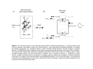
Neuronal input-state-output system Neuronal model B A 2 input EEG 1 Figure 1:A. The causal structure of an input-state-output system is defined by parameters q. It receives inputs u that can elicit changes in the states x directly (e.g. driving inputs uD, which generate post-synaptic potentials) or modulate the systems parameters (e.g. modulatory inputs uM which smoothly modify dynamics, through changes in synaptic efficacy). The MEG/EEG output y depends on both inputs and parameters. B. Neuronal model used in the simulations. Two cortical areas interact with forward and backward connections. Both areas receive a stochastic input b, which simulates ongoing activity from other brain areas. In addition, area 1 receives a stimulus a, modelled as a delta function. A single modulatory effect is considered. It simulates a stimulus-related slow modulation of extrinsic backward connectivity. The outputs of the neuronal system are the MEG/EEG signals y1 and y2 from both areas. The model used comprises three sub-populations for each area, coupled with intrinsic connections. Approximate state equations for this model are found in David & Friston 2003.
Modelling induced oscillations Figure 2 Upper Panel: Simulation of fast stimulus-related modulation of backward connectivity, using the model depicted in Figure 1B. Black curves are the responses of area 1; grey curves correspond to area 2. Time-frequency responses are shown for area 1 only. The white line, superimposed on these spectral profiles, shows the time course of the modulatory input. A. Evoked power, after averaging over trials, showing late oscillations that have been augmented by modulatory input. B. Total Power, averaged over trials. C. Induced power, normalised over frequency. Lower Panel: As for the upper panel, but here the modulatory effect has been delayed. The main difference is that low-frequency evoked components have disappeared because dynamic and structural perturbations are now separated in time and cannot interact. See main text for further details.
Transfer of energy from evoked to induced responses Figure 3: Simulation of trial-to-trial latency jitter, using the model depicted in Figure 1B. Black curves are the responses of area 1; grey curves correspond to area 2. Time-frequency responses are shown for area 1 only. A. Canonical response to a stimulus at time zero. B. Evoked responses, after averaging over trials. C. Total power, averaged over trials. D. Induced power. As predicted, high-frequency induced oscillations emerge with latency jittering (Figure 3D). This is due to the fact that trial-averaging removes high frequencies from the evoked power; as a result, they appear in the induced response.
Figure 4: Simulation of gain variations over trials. The format is the same as in Figure 3. As predicted, although gain variation has no effect on evoked power it does affect induced power, rendering it a ‘ghost’ of the evoked power. See main text for details.
Dynamic causes Evoked responses that survive averaging Evoked responses lost due to latency variations Evoked responses Induced responses Modulation of evoked responses Modulation of ongoing activity Structural causes Figure 5: Schematic illustrating the many-to-many mapping between dynamic vs.. structural causes and evoked vs.. induced responses
A B C D Figure 6: Adjusted power (3D). The format is the same as in Figure 3. As predicted, the adjusted power is largely immune to the effects of latency variation, despite the fact that evoked responses still loose their high-frequency components.