De-Noising Signals: A Wavelet Approach
310 likes | 506 Vues
De-Noising Signals: A Wavelet Approach. S. Ezekiel, W. Oblitey, R Trimble Computer Science Department Indiana University of Pennsylvania Indiana, PA 15705. Introduction. Past 3 decades– DSP fast growing fields Signal is a function of independent variable ( time, distance, position..)

De-Noising Signals: A Wavelet Approach
E N D
Presentation Transcript
De-Noising Signals: A Wavelet Approach S. Ezekiel, W. Oblitey, R Trimble Computer Science Department Indiana University of Pennsylvania Indiana, PA 15705
Introduction • Past 3 decades– DSP fast growing fields • Signal is a function of independent variable ( time, distance, position..) • Analog signal- operation done on time domain • Digital signal- both domain( time and frequency) • Multi-band spectral subtraction– Wu, Hidden Markov model– Sameti et al. --- Noise Masking algorithm – Virag---- Weighted Linear • These Models--Variable degree of success- depending on the goals and assumptions • Our goal:-develop a model to reduce various noises and improve the quality of a signal
What is Wavelet? ( Wavelet Analysis) • Wavelets are functions that satisfy certain mathematical requirements and are used to represent data or other functions • Idea is not new--- Joseph Fourier--- 1800's • Wavelet-- the scale we use to see data plays an important role • FT non local -- very poor job on sharp spikes Waveletdb10 Sine wave
History of wavelets • 1807 Joseph Fourier- theory of frequency analysis-- any 2pi functions f(x) is the sum of its Fourier Series • 1909 Alfred Haar-- PhD thesis-- defined Haar basis function---- it is compact support( vanish outside finite interval) • 1930 Paul Levy-Physicist investigated Brownian motion ( random signal) and concluded Haar basis is better than FT • 1930's Littlewood Paley, Stein ==> calculated the energy of the function 1960 Guido Weiss, Ronald Coifman-- studied simplest element of functions space called atom • 1980 Alex Grossmann (physicist) Jean Morlet( Engineer)-- broadly defined wavelet in terms of quantum mechanics • 1985 Stephane Mallat--defined wavelet for his DSP ( Ph.D. thesis) • Y. Meyer constructed first non trivial wavelet. • 1988 Ingrid Daubechies-- used Mallat work constructed set of wavelets • The name emerged from the literature of geophysics, by a route through France. The word onde led to ondelette. Translation wave led to wavelet-- by Jean Morlet
Fourier, Haar • Amplitude, time amplitude , frequency • 1965 Cooley and Tukey – Fast Fourier Transform • Haar
Wavelets Fourier Transform CWT = C( scale, position)= Scaling wave means simply Stretching (or Shrinking) it Shifting f (t) f(t-k)
Wavelet Decomposition and Reconstruction • Calculating coefficients for C at every scale– lots of work • Choose a subset– powers of 2’s dyadic scales ==> DWT • Efficient way of calculating coefficients– by using filters– defined by Mallat-- => FWT( 2 channel sub-band coder)=>decompose signal into 2 parts: approximate (low= actual content) and detail (high=flavor) • The above is called decomposition of Level 1 • This process can be iterated => signal broken down into many low-resolutions. • The procedure to reconstruct the original signal from its decomposed parts is called Reconstruction
Transforms • Transform of a signal is a new representation of that signal • Example:- signal x0,x1,x2,x3 define y0,y1,y2,y3 • Questions • 1. What is the purpose of y's • 2. Can we get back x's • Answer for 2: The Transform is invertible-- perfect reconstruction • Divide Transform in to 3 groups • 1. Lossless( Orthogonal)-- Transformed Signal has the same length • 2. Invertible (bi-orthogonal)-- length and angle may change-- no information lost • 3. Lossy ( Not invertible)--
Answer to Q1: Purpose • IT SEES LARGE vs SMALL • X0=1.2, X1= 1.0, x2=-1.0, x3=-1.2 • Y=[2.2 0 -2.2 0] • Key idea for wavelets is the concept of " SCALE" • We can take sum and difference again==> recursion => Multiresolution • Main idea of Wavelet analysis– analyze a function at different scales– mother wavelet use to construct wavelet in different scale and translate each relative to the function being analyzed • Z=[ 0 0 4.4 0 ] • Reconstruct =====>compression 4:1
Scaling function and Wavelets • corresponding to low pass--> there is scaling function • corresponding to high pass--> there is wavelet function • dilation equation--> scaling function • In terms of original low pass filters • we have • for h(0) and h(1) = 1/2 we have • the graph compressed by 2 gives and shifted by 1/2 gives • By similar way the wavelet equation
Signals and Signal Applications • There are various types of signals: • Heart Rate Variability (HRV) • Seismic Signals • Speech Signals • Noise is mixed during the data collection phase • x(t) = a(t) + d(t)
Thresholding • Transformation of an input signal to an output signal where is the Threshold value
Signal Enhancement Model • Several traditional methods, such as median filtering, averaging with various masks, and histogram have been studied and implemented • Each of these methods are designed to filter a specific type of noise, for example white, Gaussian, impulsive, additive, quantization, or multiplicative noise.
Step 1: Data Collection. A total of 57 signals were collected for study. We collected 11 speech, 14 HRV, 30 Seismic, and 2 Historic Stock Market signals. • Step 2: Resample. We added noises to test our model against. • River • car engine • air conditioner • highway traffic
Step 3: Wavelet Decomposition. Choose a wavelet. Decide the number of levels then, compute wavelet decomposition for levels. This process separates the signal into two parts, low frequency (approximate coefficients ) and high frequency (detailed coefficients). • Step 4: Remove Noises by Thresholding • Choose the threshold value and type. • Apply the thresholding technique to only the high frequency part of level • This clears out most background noise • Step 5: Reconstruction. Perform wavelet reconstruction from the approximate coefficients in step 4.
Error Measures • We used the two commonly used measure to test the quality of our signal • Root Mean Square (RMS) error • The Peak Signal-to-Noise Ratio
Heart Rate Variability (male, age 48, 8% heart disease, 24 hour sample)
We calculated the PSNR for the de-noised signals and we obtained the values 56.1370, 38.6432, 62.5, 32.568, and 27.1034 respectively. This clearly shows that our model efficiently removed the various noises. Further our model retained 98.8015%, 99.9623%, 99%, 99.47%, and 88.4015% of the original content of the signal even after removing 26.8812%, 79.5370%, 82%, 82.1181%, and 80.95% of the detail coefficients, respectively.
Conclusion • A framework using wavelet and multiresolution analysis based noise removal was presented. • This approach offers high quality and flexibility since: • Parameters can be easily modified to remove various noises • Threshold values can be automatically calculated and adjusted based on the waveform. • Although these techniques have been shown to de-noise signals, further experimental analysis is needs fine-tune the various parameters.
JPEG (Joint Photographic Experts Group) • 1. Color images ( RGB) change into luminance, chrominance, color space • 2. color images are down sampled by creating low resolution pixels – not luminance part– horizontally and vertically, ( 2:1 or 2:1, 1:1)– 1/3 +(2/3)*(1/4)= ½ size of original size • 3. group 8x8 pixels called data sets– if not multiple of 8– bottom row and right col are duplicated • 4. apply DCT for each data set– 64 coefficients • 5. each of 64 frequency components in a data unit is divided by a separate number called quantization coefficients (QC) and then rounded into integer • 6. QC encode using RLE, Huffman encoding, Arithmetic Encoding ( QM coder) • 7. Add Headers, parameters, and output the result • interchangeable format= compressed data + all tables need for decoder • abbreviated format= compressed data+ not tables ( few tables) • abbreviated format =just tables + no compressed data • DECODER DO THE REVERSE OF THE ABOVE STEPS
JPEG 2000 or JPEG Y2k • divide into 3 colors • each color is partitioned into rectangular, non-overlapping regions called tiles– that are compressed individually • A tile is compressed into 4 main steps • 1. compute wavelet transform – sub band of wavelets– integer, fp,---L+1 levels, L is the parameter determined by the encoder • 2. wavelet coeff are quantized, -- depends on bit rate • 3. use arithmetic encoder for wavelet coefficients • 4. construct bit stream– do certain region, no order • Bit streams are organized into layers, each layer contains higher resolution image information • thus decoding layer by layer is a natural way to achieve progressive image transformation and decompression
Wavelet Packet • Walsh-Hadamard transform-- complete binary tree --> wavelet packet • "Hadamard matrix"==> all entries are 1 and -1 and all rows are orthogonal-- divide two time by sqrt(2)==> orthogonal & symmetric • Compare with wavelet-- computations sums z0=0 sums y0 and y2 difference z2=4.4 x sums z1=0.4 difference y1 and y3 difference z3=0
Filters and Filter Banks • Filter is a linear time-invariant operator • It acts on input vector x --- Out put vector y is the convolution of x with a fixed vector h • h--> contains filter coefficients-- our filters are digital not analog-- h(n) are discrete time t= nT, • T is sampling period assume it is 1 here • x(n) and y(n) comes all the time t= 0, +_ 1.... • y(n) = Σh(k) x(n-k) = convolution h* x in the time domain • Filter Bank= Set of all filters • Convolution by hand--- arrange it as ordinary multiplication -- but don't carry digits from one column to another • x= 3 2 4 h= 1 5 2 • x * h = 3 17 20 24 8