Last Time

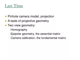
1. Last Time • Pinhole camera model, projection • A taste of projective geometry • Two view geometry: • Homography • Epipolar geometry, the essential matrix • Camera calibration, the fundamental matrix

2. Epipolar Lines epipolar plane epipolar lines epipolar lines O’ O Baseline

3. Stereo Vision • Objective: 3D reconstruction • Input: 2 (or more) images taken with calibrated cameras • Output: 3D structure of scene • Steps: • Rectification • Matching • Depth estimation

4. Rectification • We will assume images have been rectified so that epipolar lines correspond to scan lines • Image planes of cameras are parallel. • Focal points are at same height. • Focal lengths same. • Then, epipolar lines fall along the horizontal scan lines of the images • Any stereo pair can be rectified by rotating and scaling the two image planes (=homography) so that they become parallel to baseline

5. Rectification • Image Reprojection • reproject image planes onto common plane parallel to baseline • Notice, only focal point of camera really matters (Seitz)

6. Cyclopean Coordinates • Origin at midpoint between camera centers • Axes parallel to those of the two (rectified) cameras

7. Disparity • The difference is called “disparity” • dis inversely related to Z: greater sensitivity to nearby points • dis directly related to b: sensitivity to small baseline

8. Main Step: Correspondence Search • What to match? • Objects? More identifiable, but difficult to compute • Pixels? Easier to handle, but maybe ambiguous • Edges? • Collections of pixels (regions)?

9. Matching objects vs. Pixels Left Right scanline

10. Random Dot Stereogram • Using random dot pairs Julesz showed that recognition is not needed for stereo

11. Random Dot in Motion

12. Finding Matches • Under what conditions pixels can be matched? • Ignoring specularities, we can assume that matching pixels have the same brightness (constant brightness assumption) • Still, changes in gain and sensitivity may change the values of pixels • Common solution: • Use larger windows • Normalized correlation • Pros and cons: • Small window: accurate match is more likely • Large window: fewer candidates • We need a method to eliminate false matches

13. Window Size W = 3 W = 20

14. Constraining the Search • Restrict search to epipolar lines (1D search) • Use larger elements (larger windows, edges, regions) Problem: large elements may be distorted • Enforce smoothness Problem: discontinuities at object boundaries • Enforce ordering Problem: not always true

15. 1D Search

16. 1D Search • More efficient • Fewer false matches SSD error disparity

17. Ordering

18. Ordering

19. Correspondence as Optimization • Most stereo algorithms attempt to minimize a functional that usually consists of two terms: where - penalizes for quality of a match (unary) - penalizes non smooth (or even non fronto-parallel) reconstructions (binary) • Many different optimization approaches were proposed

20. Comparison of Stereo Algorithms D. Scharstein and R. Szeliski. "A Taxonomy and Evaluation of Dense Two-Frame Stereo Correspondence Algorithms," International Journal of Computer Vision,47 (2002), pp. 7-42. Scene Ground truth

21. Scharstein and Szeliski

22. Results with window correlation Window-based matching (best window size) Ground truth

23. Graph Cuts Graph cuts Ground truth

24. Stereo Algorithms We’ll briefly review several algorithms: • Dynamic programming • Minimal cut/Max flow • Space carving • Graph cut optimization

25. ?

26. 1D Methods: Dynamic Programming • Discretize the 3-D space • Find the correct curve at every slice (A slice = epipolar plane)

27. Dynamic programming Find correspondences of each epipolar line separately

28. Dynamic programming

29. Dynamic programming How do we find the best curve? • Assign weight of all edges insertion match deletion

30. Dynamic programming How do we find the best curve? • Assign weight of all edges • Find shortest path • Dijkstra insertion match deletion

31. Results

32. Dynamic programming Advantages • Simple, efficient • Globally optimal Disadvantages • Each slice computed independently (smoothness is not enforced between slices) • Problems due to discretization (tilted planes)

33. Min Cut/Max Flow

34. Min Cut/Max Flow

35. Min Cut/Max Flow

36. Min Cut/Max Flow

37. Min Cut/Max Flow Objective: find the optimal cut using all the slices simultaneously.

38. Min Cut/Max Flow Construct a graph: • Every voxel (3-D point in space) is a node • Every node is connected to its 6 neighbors

39. Min Cut/Max Flow Weights on the edges: • Data cost: change in pixel value data data

40. Min Cut/Max Flow Weights on the edges: • Data cost: change in pixel value • Smoothness cost: change in depth smooth smooth smooth smooth

41. Min Cut/Max Flow Weights on the edges: • Data cost: change in pixel value • Smoothness cost: change in depth

42. … … Min Cut/Max Flow Source • Add source and sink • Find min cut ∞ ∞ Sink

43. Min Cut/Max Flow Data penalty Smoothness penalty

44. Results Input Min cut Dynamic programming

45. Min Cut/Max Flow Advantages • All slices are optimized simultaneously • Efficient Disadvantages • Extension to multi-camera is difficult • Discretization

46. Space Carving • Multi-view stereo • Every point in space corresponds to a match in the images • Compute data term for each match

47. Space Carving • Multi-view stereo • Every point in space corresponds to a match in the images • Compute data term for each match (“photo-consistency”)

48. Space Carving • Dynamic data term (taking occlusion into account) • Order of sweep is important

49. Space Carving

50. Space Carving • Done for all slices simultaneously