Understanding Binomial Distribution: Key Concepts and Applications
Learn about the binomial distribution, random variables, probability functions, and its applications in various scenarios like political polls, coin tossing, and more. This guide covers the summarization and probability structures related to binomial distributions.

Understanding Binomial Distribution: Key Concepts and Applications
E N D
Presentation Transcript
Last Time • Administrative Matters – Blackboard … • Random Variables • Abstract concept • Probability distribution Function • Summarizes probability structure • Sum to get any prob. • Binomial Distribution
Reading In Textbook Approximate Reading for Today’s Material: Pages 311-317, 327-331, 372-375 Approximate Reading for Next Class: Pages 377-381, 385-391, 488-491
Binomial Distribution Setting: n independent trials of an experiment with outcomes “Success” and “Failure”, with P{S} = p.
Binomial Distribution Setting: n independent trials of an experiment with outcomes “Success” and “Failure”, with P{S} = p. Say X = #S’s has a “Binomial(n,p) distribution”, and write “X ~ Bi(n,p)”
Binomial Distribution Setting: n independent trials of an experiment with outcomes “Success” and “Failure”, with P{S} = p. Say X = #S’s has a “Binomial(n,p) distribution”, and write “X ~ Bi(n,p)” • Called “parameters” (really a family of distrib’ns, indexed by n & p)
Binomial Distribution E.g. Sampling with replacement • “Experiment” is “draw a sample member” • “S” is “vote for Candidate A” • “p” is proportion in population for A (note unknown, and goal of poll) • Independent? (since with replacement)
Binomial Distribution E.g. Sampling with replacement • “Experiment” is “draw a sample member” • “S” is “vote for Candidate A” • “p” is proportion in population for A (note unknown, and goal of poll) • Independent? (since with replacement) X = #(for A) has a Binomial(n,p) dist’n
Binomial Distribution E.g. Sampling without replacement • Draws are dependent Result of 1st draw changes probs of 2nd draw • P(S) on 2nd draw is no longer p (again depends on 1st draw) X = #(for A) is NOT Binomial
Binomial Distribution E.g. Sampling without replacement • Draws are dependent Result of 1st draw changes probs of 2nd draw • P(S) on 2nd draw is no longer p (again depends on 1st draw) X = #(for A) is NOT Binomial (although approximately true for large pop’n)
Binomial Distribution Models much more than political polls: E.g. Coin tossing (recall saw “independence” was good) E.g. Shooting free throws (in basketball) • Is p always the same? • Really independent? (turns out to be OK)
Binomial Prob. Dist’n Func. • Summarize all prob’s for X ~ Bi(n,p)
Binomial Prob. Dist’n Func. • Summarize all prob’s for X ~ Bi(n,p) • By function:
Binomial Prob. Dist’n Func. • Summarize all prob’s for X ~ Bi(n,p) • By function: Recall: • Sum over this for any prob. about X
Binomial Prob. Dist’n Func. • Summarize all prob’s for X ~ Bi(n,p) • By function: Recall: • Sum over this for any prob. about X • Avoids doing complicated calculation each time want a prob.
Binomial Prob. Dist’n Func. Repeat “experiment” (S or F) n times
Binomial Prob. Dist’n Func. Repeat “experiment” (S or F) n times • Outcomes “Success” or “Failure”
Binomial Prob. Dist’n Func. Repeat “experiment” (S or F) n times • Outcomes “Success” or “Failure” • Independent repetitions • Let X = # of S’s (count S’s)
Binomial Prob. Dist’n Func. Repeat (S or F) n times (ind.), let X = # of S’s
Binomial Prob. Dist’n Func. Repeat (S or F) n times (ind.), let X = # of S’s P[X = x] = Desired probability distribution function
Binomial Prob. Dist’n Func. Repeat (S or F) n times (ind.), let X = # of S’s P[X = x] = Depends on particular draws, So expand in those terms, and use Big Rules of Probability
Binomial Prob. Dist’n Func. Repeat (S or F) n times (ind.), let X = # of S’s P[X = x] = P[(S1&…&Sx&Fx+1&…&Fn) or …] • For “S on 1st draw”, “S on x-th draw”, …
Binomial Prob. Dist’n Func. Repeat (S or F) n times (ind.), let X = # of S’s P[X = x] = P[(S1&…&Sx&Fx+1&…&Fn) or …] • For “S on 1st draw”, “S on x-th draw”, … • One possible ordering of S,…,S,F,…,F where: x of these n-x of these
Binomial Prob. Dist’n Func. Repeat (S or F) n times (ind.), let X = # of S’s P[X = x] = P[(S1&…&Sx&Fx+1&…&Fn) or …] • For “S on 1st draw”, “S on x-th draw”, … • One possible ordering of S,…,S,F,…,F • This includes all other orderings (very many, but we can think of them)
Binomial Prob. Dist’n Func. Repeat (S or F) n times (ind.), let X = # of S’s P[X = x] = P[(S1&…&Sx&Fx+1&…&Fn) or …] Next decompose with and – or – not Rules of Probability
Binomial Prob. Dist’n Func. Repeat (S or F) n times (ind.), let X = # of S’s P[X = x] = P[(S1&…&Sx&Fx+1&…&Fn) or …] = = P[(S1&…&Sx&Fx+1&…&Fn)] + … • Disjoint OR rule [“or” add]
Binomial Prob. Dist’n Func. Repeat (S or F) n times (ind.), let X = # of S’s P[X = x] = P[(S1&…&Sx&Fx+1&…&Fn) or …] = = P[(S1&…&Sx&Fx+1&…&Fn)] + … • Disjoint OR rule [“or” add] (recall “no overlap”)
Binomial Prob. Dist’n Func. Repeat (S or F) n times (ind.), let X = # of S’s P[X = x] = P[(S1&…&Sx&Fx+1&…&Fn) or …] = = P[(S1&…&Sx&Fx+1&…&Fn)] + … = P(S1)…P(Sx)P(Fx+1)…P(Fn) + … • Independent AND rule [“and” mult.]
Binomial Prob. Dist’n Func. Repeat (S or F) n times (ind.), let X = # of S’s P[X = x] = P[(S1&…&Sx&Fx+1&…&Fn) or …] = = P[(S1&…&Sx&Fx+1&…&Fn)] + … = P(S1)…P(Sx)P(Fx+1)…P(Fn) + … = since p = P[S] since (1-p) = P[F]
Binomial Prob. Dist’n Func. Repeat (S or F) n times (ind.), let X = # of S’s P[X = x] = P[(S1&…&Sx&Fx+1&…&Fn) or …] = = P[(S1&…&Sx&Fx+1&…&Fn)] + … = P(S1)…P(Sx)P(Fx+1)…P(Fn) + … = since x = #S’s since (n-x) = #F’s
Binomial Prob. Dist’n Func. Repeat (S or F) n times (ind.), let X = # of S’s P[X = x] = P[(S1&…&Sx&Fx+1&…&Fn) or …] = = P[(S1&…&Sx&Fx+1&…&Fn)] + … = P(S1)…P(Sx)P(Fx+1)…P(Fn) + … = = #(terms) since all of these are the same, just count
Binomial Prob. Dist’n Func. Repeat (S or F) n times (ind.), let X = # of S’s P[X = x] = #(terms) # ways to order S …S F …F
Binomial Prob. Dist’n Func. Repeat (S or F) n times (ind.), let X = # of S’s P[X = x] = #(terms) # ways to order S …S F …F Approach: have “n slots”
Binomial Prob. Dist’n Func. Repeat (S or F) n times (ind.), let X = # of S’s P[X = x] = #(terms) # ways to order S …S F …F Approach: have “n slots” “choose x of them to in which to put S”
Binomial Prob. Dist’n Func. Repeat (S or F) n times (ind.), let X = # of S’s P[X = x] = #(terms) # ways to order S …S F …F Approach: have “n slots” “choose x of them to in which to put S” thus have #(terms) =
Binomial Prob. Dist’n Func. Repeat (S or F) n times (ind.), let X = # of S’s P[X = x] = #(terms) = general formula that works for all n, p, x
Binomial Prob. Dist’n Func. Repeat (S or F) n times (ind.), let X = # of S’s P[X = x] = #(terms) = = Binomial Probability Distribution Function (for any n and p)
Binomial Prob. Dist’n Func. Repeat (S or F) n times (ind.), let X = # of S’s More complete representation
Binomial Prob. Dist’n Func. Repeat (S or F) n times (ind.), let X = # of S’s More complete representation But generally assume is understood, & write
Binomial Prob. Dist’n Func. Application of: For X ~ Bi(n,p) • Compute any probability for X • By summing over appropriate values
Application of Bi. Pro. Dist. Fun. Application of: E.g.: A system fails if any 3 of 5 independent components fail
Application of Bi. Pro. Dist. Fun. Application of: E.g.: A system fails if any 3 of 5 independent components fail • Common setup in Reliability Theory
Application of Bi. Pro. Dist. Fun. Application of: E.g.: A system fails if any 3 of 5 independent components fail • Common setup in Reliability Theory • Used when things “really need to work” • E.g. aircraft components
Application of Bi. Pro. Dist. Fun. Application of: E.g.: A system fails if any 3 of 5 independent components fail If each component works 99% of time,
Application of Bi. Pro. Dist. Fun. Application of: E.g.: A system fails if any 3 of 5 independent components fail If each component works 99% of time, how likely is the system to break down?
Application of Bi. Pro. Dist. Fun. Application of: E.g.: Sys. F if 3 of 5 F, each works 99% time, how likely is the system to break down?
Application of Bi. Pro. Dist. Fun. Application of: E.g.: Sys. F if 3 of 5 F, each works 99% time, how likely is the system to break down? Let X = #F’s
Application of Bi. Pro. Dist. Fun. Application of: E.g.: Sys. F if 3 of 5 F, each works 99% time, how likely is the system to break down? Let X = #F’s, model X ~ Bi(5,0.01)
Application of Bi. Pro. Dist. Fun. Application of: E.g.: Sys. F if 3 of 5 F, each works 99% time, how likely is the system to break down? Let X = #F’s, model X ~ Bi(5,0.01) • Recall n = # of trials (repeats of experim’t)
Application of Bi. Pro. Dist. Fun. Application of: E.g.: Sys. F if 3 of 5 F, each works 99% time, how likely is the system to break down? Let X = #F’s, model X ~ Bi(5,0.01) • Components assumed independent
Application of Bi. Pro. Dist. Fun. Application of: E.g.: Sys. F if 3 of 5 F, each works 99% time, how likely is the system to break down? Let X = #F’s, model X ~ Bi(5,0.01) • Recall p = P(“S”), on each trial (works 99%, so fails 1%)

