Advanced Processing Techniques for GOCE Gravity Field Data: Methods and Results
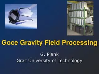
This document outlines advanced methods for processing gravity field data from the GOCE satellite, focusing on the core solver, tuning machine, and filter design approaches. Utilizing time-wise data inspection and semi-analytical methods (QL-GFA), we address challenges such as data gaps and the change of the reference frame, ensuring high accuracy in measurements. The rigorous solution strategy (DNA) effectively handles gaps and provides reliable results for gravitational field analysis, with storage requirements and computational demands detailed. Future steps include investigations on noise levels in gradiometric data.

Advanced Processing Techniques for GOCE Gravity Field Data: Methods and Results
E N D
Presentation Transcript
Goce Gravity Field Processing G. Plank Graz University of Technology
Core Solver • Tuning machine (pcgma) • Filter design • Data inspection Time-wise approach (TUG / TUM / ITG) • QL-GFA (semi-analytical) • Check L1B data • Noise PSD of the SGG data Approximative Very fast (minutes) Handles partial data sets Approximative Fast (hours) Uses recursive filters Average (days) ~15 GB RAM (D/O 250) Parallel HW needed • Final solver (DNA) • Rigorous solution • Full var.-cov. matrix
Two problems Change of the reference frame of the observations RERF GRF Non-continuous data stream of the observations Data gaps
RERF GRF Problem definition Due to the loss of the FEEPs, attitude control is now performed by magnetic torquers. Highest accuracy of the gradiometer is in the GRF. Rotation of the base functions has to be performed. Rotating the measurement tensor affects all the components. A mixture of accurate and inaccurate elements has to be avoided.
Additional rotations around z-, and x-axes with a magnitude varying between 2° and 3°. Superposed noise to simulate the accuracy of the star tracker with a magnitude of ± 5 arcminutes or ± 5 arcseconds.
RERF GRF noise free rotation RMS = 0.6 mgal RMS = 0.6 mgal
±5 arcminutes±5 arcseconds RMS = 1.7 mgal RMS = 0.6 mgal
Change of the reference frame of the observations yields no loss of accuracy of the final products (and derived quantities), as far as the rotation angles are known with an accuracy of some arcseconds.
Data gaps Problem definition In using digital recursive filters, the „memory“ of the filter has to be filled with appropriate values (e.g. the last observations) warmup phase. If this warmup phases are ignored, a direct effect is mapped on the resulting coefficients, and derived quantities (e.g. geoid heights).
Gap: ~7 % of the orbit data varying length between 1 and 100 Data Points (~ 8 min) No gaps RMS = 0.6 mgal
No gapsignore gaps RMS = 0.6 mgal RMS = 5.8 mgal
Data gaps strategies Two possibilities to reduce the influence of data gapson the used filter: • Start of a new warmup phase after each gap. Pro: no „external“ information is included in the system. Con: additional observations after the gap are not used for the final solution. • Usage of simulated observations in the gaps to fill the „memory“ of the filter with appropriate values. Pro: no observations outside of the gaps are lost. Con: „external“ information is included also in the final solution.
Original observations EGM96 RMS = 0.6 mgal RMS = 1.6 mgal
Original observations QL-GFA (interpolated) RMS = 0.6 mgal RMS = 0.6 mgal
Original observations new warmup RMS = 0.6 mgal RMS = 0.7 mgal
Simulation „Reality“ • 59 days repeat orbit, sampling interval 5s (data-set D) • Main diagonal elements of SGG measurement tensor • Based on OSU91a, lmax = 250 • size of full normal equation matrix ~15 Gbyte • Realistic colored noise • SST normal equations (lmax = 80) included (energy balance approach)
OSU91a vs. DNA RMS = 5.6 mgal
Time behavior Storage requirements One measurement phase of the GOCE satellite (6 months / 1s sampling) can be processed by the rigorous strategy (DNA) within one month!
Conclusions • The new reference frame of the observations (GRF) does not impact the overall performance of GOCE (as far as the star tracker is accurate enough) • Data gaps can be handled by a combination of two different solution strategies (QL-GFA + DNA) • The DNA approach is able to deliver the results in reasonable time Outlook • Additional investigations due to the new noise level of the gradiometer are needed (official test data sets!) Thank you