Hypothesis t esting. Parametric t ests

Hypothesis testing.Parametric tests Georgi Iskrov, MBA, MPH, PhD Department of Social Medicine

Outline • Statistical inference • Hypothesistesting • Type I andtype II errors • Student t test • ANOVA • Parametric vsnon-parametric tests

Importance of biostatistics • Diabetestype 2 study • Experimental group: Meanbloodsugarlevel: 103 mg/dl • Control group: Mean blood sugar level: 107 mg/dl • Pancreaticcancerstudy • Experimental group: 1-year survivalrate: 23% • Control group: 1-year survivalrate: 20% Isthere a difference? Statistics are needed to quantify differences that are too small to recognize through clinical experience alone.

Statistical inference • Diabetes type 2 study • Experimental group: Mean blood sugar level: 103 mg/dl • Control group: Mean blood sugar level: 107 mg/dl • Increased sample size: • Diabetes type 2 study • Experimental group: Mean blood sugar level: 99 mg/dl • Control group: Mean blood sugar level: 112 mg/dl

Statistical inference • Compare the mean between 2 samples/ conditions • if 2 means are statistically different, then the samples are likely to be drawn from 2 different populations, ie they really are different µ1 µ2 X1 X2

Statistical inference • Diabetestype 2 study • Experimental group: Meanbloodsugarlevel: 103 mg/dl • Control group: Mean blood sugar level: 107 mg/dl • Increasedsamplesize: • Diabetestype 2 study • Experimental group: Meanbloodsugarlevel: 105 mg/dl • Control group: Mean blood sugar level: 106 mg/dl

Statistical inference • Compare the mean between 2 samples/ conditions • if 2 samples are taken from the same population, then they should have fairly similar means X1 µ X2

Hypothesis testing • The general idea of hypothesis testing involves: • Making an initial assumption; • Collecting evidence (data); • Based on the available evidence (data), deciding whether to reject or not reject the initial assumption. • Every hypothesis test — regardless of the population parameter involved — requires the above three steps.

Criminal trial • Criminal justice system assumes the defendant is innocent until proven guilty. That is, our initial assumption is that the defendant is innocent. • In the practice of statistics, we make our initial assumption when we state our two competing hypotheses – the null hypothesis (H0) and the alternative hypothesis (HA). Here, our hypotheses are: • H0: Defendant is not guilty (innocent) • HA: Defendant is guilty • In statistics, we always assume the null hypothesis is true. That is, the null hypothesis is always our initial assumption.

Null hypothesis – H0 • This is the hypothesis under test, denoted as H0. • The null hypothesis is usually stated as the absence of a difference or an effect. • The null hypothesis says there is no effect. • The null hypothesis is rejected if the significance test shows the data are inconsistent with the null hypothesis.

Alternative hypothesis – H1 • This is the alternative to the null hypothesis. It is denoted as H', H1, or HA. • It is usually the complement of the null hypothesis. • If, for example, the null hypothesis says two population means are equal, the alternative says the means are unequal

Criminal trial • The prosecution team then collects evidence with the hopes of finding sufficient evidence to make the assumption of innocence refutable. • In statistics, the data are the evidence. • The jury then makes a decision based on the available evidence: • If the jury finds sufficient evidence — beyond a reasonable doubt — to make the assumption of innocence refutable, the jury rejects H0 and deems the defendant guilty. We behave as if the defendant is guilty. • If there is insufficient evidence, then the jury does not reject H0. We behave as if the defendant is innocent.

Making the decision • Recall that it is either likely or unlikely that we would observe the evidence we did given our initial assumption. • If it is likely, we do not reject the null hypothesis. • If it is unlikely, then we reject the null hypothesis in favor of the alternative hypothesis. • Effectively, then, making the decision reduces to determining likely or unlikely.

Making the decision • In statistics, there are two ways to determine whether the evidence is likely or unlikely given the initial assumption: • We could take the critical value approach (favored in many of the older textbooks). • Or, we could take the P-value approach (what is used most often in research, journal articles, and statistical software).

Making the decision • Suppose we find a difference between two groups in survival: • patients on a new drug have a survival of 15 months; • patients on the old drug have a survival of 18 months. • So, the difference is 3 months. • Do we accept or reject the hypothesis of no true difference between the groups (the two drugs)? • Is a difference of 3 a lot, statistically speaking – a huge difference that is rarely seen? • Or is it not much – the sort of thing that happens all the time?

Probability • A measure of the likelihood that a particular event will happen. • It is expressed by a value between 0 and 1. • First, note that we talk about the probability of an event, but what we measure is the rate in a group. • If we observe that 5 babies in every 1000 have congenital heart disease, we say that the probability of a (single) baby being affected is 5 in 1000 or 0.005. 0.0 1.0 Cannot happen Sure to happen

Making the decision • A statistical test tells you how often youwould get a difference of 3, simply by chance, if the null hypothesis is correct – no real difference between the two groups. • Suppose the test is done and its result is that P = 0.32. This means that youwould get a difference of 3 quite often just by the play of chance – 32 times in 100 – even when there is in reality no true difference between the groups.

Making the decision • A statistical test tells you how often you’d get a difference of 3, simply by chance, if the null hypothesis is correct – no real difference between the two groups. • On the other hand if we did the statistical analysis and P = 0.0001, then we say that you’d only get a difference as big as 3 by the play of chance 1 time in 10 000. That’s so rarely that we want to reject our hypothesis of no difference: there is something different about the new therapy.

Hypothesis testing • Somewhere between 0.32 and 0.0001 we may not be sure whether to reject the null hypothesis or not. • Mostly we reject the null hypothesis when, if the null hypothesis were true, the result we got would have happened less than 5 times in 100 by chance. This is the conventional cutoff of 5% or P < 0.05. • This cutoff is commonly used but it’s arbitrary i.e. no particular reason why we use 0.05 rather than 0.06 or 0.048 or whatever.

Hypothesis testing

Type I and II errors A type I error is the incorrect rejection of a true null hypothesis (also known as a false positive finding). The probability of a type I error is denoted by the Greek letter  (alpha). A type II error is incorrectly retaining a false null hypothesis (also known as a false negative finding). The probability of a type II error is denoted by the Greek letter  (beta).

Level of significance Level of significance (α) – the threshold for declaring if a result is significant. If the null hypothesis is true, α is the probability of rejecting the null hypothesis. α is decided as part of the research design, while P-value is computed from data. α = 0.05 is most commonly used. Small α value reduces the chance of Type I error, but increases the chance of Type II error. Trade-off based on the consequences of Type I (false-positive) and Type II (false-negative) errors.

Power Power – the probability of rejecting a false null hypothesis. Statistical power is inversely related to β or the probability of making a Type II error (power is equal to 1 – β). Power depends on the sample size, variability, significance level and hypothetical effect size. You need a larger sample when you are looking for a small effect and when the standard deviation is large.

Common misconceptions • P-value is different from the level of significance α. P-value is computed from data, while α is decided as part of the experimental design. • P-value is not the probability of the null hypothesis being true. P-value answers the following question: If the null hypothesis is true, what is the chance that random sampling will lead to a difference as large as or larger than observed in the study. • A statistically significant result does not necessarily mean that the finding is clinically important. Look at the size of the effect and its precision. • Lack of difference may be a meaningful result too!

Choosing a statistical test Choice of a statistical test depends on: Level of measurement for the dependent and independent variables; Number of groups or dependent measures; Number of units of observation; Type of distribution; The population parameter of interest (mean, variance, differences between means and/or variances).

Choosing a statistical test • Multiple comparison – two or more data sets, which should be analyzed • repeated measurements made on the same individuals; • entirely independent samples. • Degrees of freedom – the number of scores, items, or other units in the data set, which are free to vary • One- and two tailed tests • one-tailed test of significance used for directional hypothesis; • two-tailed tests in all other situations. • Sample size – number of cases, on which data have been obtained • Which of the basic characteristics of a distribution are more sensitive to the sample size?

Student t-test

1-sample t-test • Comparison of sample mean with a population mean • It is known that the weight of young adult male has a mean value of 70.0 kg with a standard deviation of 4.0 kg. Thus the population mean, µ= 70.0 and population standard deviation, σ= 4.0. • Data from random sample of 28 males of similar ages but with specific enzyme defect: mean body weight of 67.0 kg and the sample standard deviation of 4.2 kg. • Question: Whether the studied group have a significantly lower body weight than the general population?

2-sample t-test Aim: Compare two means Example: Comparing pulse rate in people taking two different drugs Assumption: Both data sets are sampled from Gaussian distributions with the same population standard deviation Effect size: Difference between two means Null hypothesis: The two population means are identical Meaning of P value: If the two population means are identical, what is the chance of observing such a difference (or a bigger one) between means by chance alone?

Paired t-test Aim: Compare a continuous variable before and after an intervention Example: Comparing pulse rate before and after taking a drug Assumption: The population of paired differences is Gaussian Effect size: Mean of the paired differences Null hypothesis: The population mean of paired differences is zero Meaning of P value: If there is no difference in the population, what is the chance of observing such a difference (or a bigger one) between means by chance alone?

One-way ANOVA Aim: Compare three or more means Example: Comparing pulse rate in 3 groups of people, each group taking a different drug Assumption: All data sets are sampled from Gaussian distributions with the same population standard deviation Effect size: Fraction of the total variation explained by variation among group means Null hypothesis: All population means are identical Meaning of P value: If the population means are identical, what is the chance of observing such a difference (or a bigger one) between means by chance alone?

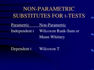
Parametric andnon-parametric tests Parametric test – the variable we have measured in the sample is normally distributed in the population to which we plan to generalize our findings Non-parametric test – distribution free, no assumption about the distribution of the variable in the population

Parametric andnon-parametric tests

Hypothesis t esting. Parametric t ests