Download
1 / 75
760 likes | 956 Vues
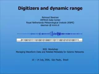
Digitizers and dynamic range Reinoud Sleeman ORFEUS Data Center Royal Netherlands Meteorological Insitute (KNMI) sleeman @ knmi.nl IRIS Workshop Managing Waveform Data and Related Metadata for Seismic Networks 10 – 14 July, 2006, Sao Paulo, Brazil.

E N D
Digitizers and dynamic range Reinoud Sleeman ORFEUS Data Center Royal Netherlands Meteorological Insitute (KNMI) sleeman @ knmi.nl IRIS Workshop Managing Waveform Data and Related Metadata for Seismic Networks 10 – 14 July, 2006, Sao Paulo, Brazil
Seismic background noise power spectral density Station Heimansgroeve (HGN), Netherlands 2002:302-309, 2003:029-043 Instrument corrected PSD (Peterson, USGS)
Possible contributing sources: • Barometric pressure variations (ground tilt, elastic response ) • Temperature variations • Instrument response (true vs. nominal) • Installation conditions (background noise) • Quantization noise of digitizer • Sensor self-noise :
How do we get a digital (bit stream) representation • from an analog signal ? • How accurate is the representation ? • Does the recording system bias the digital data ? • What does ‘dynamic range’ mean and how must we • interpret these numbers (e.g. 145 dB, 24 bits …) given • by vendors ? • How can we measure/quantify the dynamic range ? • What information about the recording system is useful • or important to know for seismologists and needs • therefore to be stored as metadata ?
Digital seismograph system datalogger
Quantization is the process of approximating a continuous range of values by a relatively-small set of discrete symbols or integer values A common use of quantization is in the conversion of a sampled continuous signal into a digital signal by quantizing. Both of these steps (sampling and quantizing) are performed in analog-to-digital converters with the quantization level specified in bits.
Dynamic range of a N-bit digitizer – some theory: Quantization: Variance of error: Quantization levels: N-bit ADC Dynamic range: (Bennett, 1948)
Dynamic range of a N-bit digitizer – some theory: Quantization: Variance of error: Quantization levels: N-bit ADC Dynamic range: (Bennett, 1948) Sine wave (amp A): 6 dB per bit Dynamic range digitizer:
The resolution of the converter indicates the number of discrete values • it can produce over the range of voltage values. It is usually expressed in • bits. • Example: • Full scale RMS measurement range = 0 to 10 volts • ADC resolution is 12 bits: 212 = 4096 quantization levels • ADC voltage resolution is: (10-0)/4096 = 0.00244 volts = 2.44 mV • SNR = 20 log ( 10 / 2.44 10-3 ) ≈ 72 dB
Oversampling PSD vs. sampling rate • In an ideal digitizer (assuming white digitizer noise) the quantization • noise power is uniformly distributed between [0 – fNYQ] Hz. • The noise power is independent of the sampling rate. • For higher sampling rates the power spread over a wider frequency range, so • decreasing the power spectral density (so decreasing the quantization error) ! • Higher sampling rate improves the accuracy of the estimate of the (analog) • input signal.
Oversampling T = sampling interval (s) PSD of quantization error depends on the (initial) sampling rate, … so also the dynamic range !
Oversampling • oversampling factor 4 leads to increase of SNR of ~ 6 dB (or 1 bit) • 1-bit ADC with 256x oversampling achieves a resolution of 4 bits; • to achieve 16 bits resolution you must oversample with factor 4^16 • (~ 4e9), which is not realizable ! • this problem is overcome by the delta-sigma converter with the • property of noise shaping, to enable a gain of more than 6 dB for • each factor of 4x oversampling.
Delta-Sigma Analog-Digital (A/D) Modulator (one-bit noise shaping converter) Comperator: ADC or quantizer Feedback: average of y follows the average of x Integrator: accumulates the quantization error e over time Pulse train: pulse density representation of x
Relatively low clock speed digitizer Analog input 1 Digital “pulse train” output 0
Relatively high clock speed digitizer Analog input 1 Digital “pulse train” output 0
Delta-Sigma Digitizer ei si ui q(ui) xi Noise shaping 2-nd order:
Assumption: quantization noise is white noise with feedback PSD noise without feedback 0 100 (Hz) 32000 The feedback loop in the quantizer shapes (differentiates) the quantization noise, with the result of smaller quantization noise at lower frequencies at the price of larger quantization noise at higher frequencies. Noise shaping does not change the total noise power, but its distribution.
Dithering When the signal has the same order of amplitude as the quantization error, the error can repeat and correlate to the signal. Dithering is the process of adding random noise to the digitizer to decorrelate the quantization error and the signal. random noise [ 0 - 0.5 LSB]
…. also used in digital images without dithering with dithering
Differential Input • high common-mode impedance (external noise rejection) • low differential impedance
Differential ADC Input • doubles the dynamic range 5 V 5 V 0 V 5 V 10 V -5 V
Delta-Sigma Digitizer: summary • Oversampling: quantization noise PSD reduction • Feedback: noise shaping, quantization noise PSD reduction • Feedback order: higher order, improved noise reduction • Dithering: decorrelates signal and quantization noise • (may reduce quantization noise) • Differential input: increases dynamic range • Decimation decrease sample rate (using digital filters (FIR)) Improved resolution (reduced quantization error) and dynamic range at a lower effective sampling rate
How do we represent and measure the dynamic range of a digitizer ? Clip level (sine wave) No gain ranging: High dynamic range, High resolution Gain ranging: High dynamic range, Low resolution Amplitude 1/f Instrument noise level (quantization error noise) Frequency
Choosing a spectral measure for data analysis • How to quantify the amplitude level and frequency content of noise and a sine wave in terms of its frequency spectrum ? • deterministic signal: stationary, sine waves • power [V2], or RMS amplitude [V] • random: continuous, stationary, non-deterministic, noise • power spectral density [V2/Hz] • transients: finite time, earthquake signal • power [V2], or RMS amplitude [V] High resolution analysis Low resolution analysis
The total RMS noise power in a specific band is the integral of the power spectral density across that band You have to specify the bandwidth if you use RMS values to specify the dynamic range !
Possible representations of dynamic range • ratio of maximum noise peak amplitude and clip level • specify frequency band (e.g. 1/2 octave or 1/6 decade) • (RMS full scale sine ) / (RMS noise ) • Bennett, 1948: • Power Spectral Density graph, as function of frequency
Ways to measure instrumental noise of digitizers (and seismic sensors) • How can we determine the dynamic range from the measurements ? • Does the quantization error increases during quantizing a seismic signal ? • 50 ohm shortened input recording • common input recording • coherency analysis of 2 channels • coherency analysis of 3 channels
Quanterra Q4120: shortened input • 50 ohm shortened input recording (1 Count ≈ 2.38 ·10-6 V gain) • SNR = (RMS full scale sine) / (RMS noise) Vpp = 40 V Vrms = 14.1 V dt = 0.05 s 0.01 – 8 Hz: RMS noise 0.8 uV (measured) 143.8 dB (rel to 1 V 2 ) @ 20 sps 23.6 bits
Quanterra Q4120: shortened input • 50 ohm shortened input recording (1 Count ≈ 2.38 ·10-6 V gain) • RMS noise vs. frequency graph ( by integrating the PSD over 1/6 decade bandwidth )
Quanterra Q4120: shortened input • 50 ohm shortened input recording (1 Count ≈ 2.38 ·10-6 V gain) • RMS noise vs. frequency graph ( by integrating the PSD over 1/6 decade bandwidth ) PSD estimation (Welch, 1967): • 50 % overlapping time sections (~ 800 sec) • tapering (normalized Hanning window) • Fourier transform • Periodogram: • averaging over the number of time sections • PSD smoothing over 1/10 th of decade
1 V ) ~ 145 dB dithering ? Shorted input noise RMS
Quanterra Q4120: common input recording (e.g. STS-2) • coherency analysis (conventional, using 2 channels; Holcomb, 1989) • coherency analysis (new technique, using 3 channels; Sleeman et. al., 2006) Holcomb, L. G., A direct method for calculating instrument noise levels in side-by-side seismometer evaluations. U.S. Geol. Surv., Open-File Report 89-214 (1989) Sleeman, R., A. van Wettum and J. Trampert. Three-channel correlation analysis: a new technique to measure instrumental noise of digitizers and seismic sensors. Bull. Seism. Soc. Am., 96, 1, 258-271 (2006)
The mathematical description of the three-channel linear system shows that we can estimate, solely from the output recordings: • the ratio of the transfer functions between the channels • the noise spectrum for each channel We do not need to know the transfer function, or its accuracy, as is required in the 2-channel model !
Synthetic test: 2-channel versus 3-channel method n1: rms = 1.0 n2: rms = 1.09 n3: rms = 0.94 dt = 0.025 s s: rms = 1.0 H1 = 1000 H2 = 1030 (3%) H3 = 1200 (20%) SNR ≈ 60 dB output noise (2-channel method: H1, H2) noise (MCCA)
Synthetic test: ratios between transfer functions theoretical H1/H2 H2/H3 H1/H3
Synthetic test: performance vs. SNR output noise (MCCA)
Three-channel technique: • direct method for estimating system noise and transfer function based on the recordings only • no a-priori information required about transfer functions • method not sensitive for errors in gain • better transfer ratio estimations with higher SNR • works up to 120 dB SNR