The Big-O
The Big-O. CS 263. Big O Notation. Classification of algorithm against a model pattern Each model demonstrate the performance scalability of an algorithm Sorting algorithms might have different model patterns Depending on the number of records sorted, one model might work better than another

The Big-O
E N D
Presentation Transcript
The Big-O CS 263
Big O Notation • Classification of algorithm against a model pattern • Each model demonstrate the performance scalability of an algorithm • Sorting algorithms might have different model patterns • Depending on the number of records sorted, one model might work better than another • However.. An increase in records would invoke high overhead in processing at some point • A search of records would assume that the record is the last to be found (or non-existent), a worst-case scenario • Noted as O(N) • A 25 record search would take five times as long as the 5 record search
Big O • The presumption is that we’re talking about speed/performance • We could also be concerned with other resources • Memory utilization • Disk trashing • Depending on the resource we’re targeting, the algorithm might change • Slower algorithm (time) vs. memory consumption
Big O • Constants and variables • Algorithm 1 • Compare each array element against every other element for my $i (0 .. $#array) { for my $j (0 .. $#array) { next if $j == $i; # Compare $i, $j } } • O(N^2) • Algorithm 2 • Optimized algorithm, cuts run time in half for my $i (0 .. $#array - 1) { for my $j ($i + 1 .. $#array) { # Compare $i, $j } } • The notation is NOT O(N2/2), but still O(N2) • The “divide by 2” remains constant regardless of input size
Big O • Big O will not care if you purchase more RAM • It’s THEORY • So why bother? • It serves as an indicator of which algorithm to use when you consider your circumstances • Big O servers as a “limiting behavior” of a function • An upper bound of performance • Big O also referred to as • Landau notation • Bachmann-Landau notation • Asymptotic notation
Common Orders of Growth • O(1) No growth curve • Performance is independent of the size of the data set • O(N) • Performance is directly proportional to the size of the data set • O(N+M) • Two data sets combined, and that determines performance • O(N2) • Each element of a set requires to be processed against all others. Bubble sorts are in this category • O(N*M) • Each element of one data set is processed against each element of another data set • Set of regular expressions needs to be processed against a text file • O(N3) • Nested looping going on here…
Common Orders of Growth • O(log N) and O(N log N) • Data set is “iteratively partitioned” (example… balanced binary tree) • Unbalanced trees are O(N2) to build and O(N) to search • The O(log N) refers to the number of times you can partition a set in half iteratively • Log2N grows slowly (doubling N has a small effect) and the curve flattens out • Building the tree is more expensive
Big O • Scaling order • O(1) • O(log N) • O(N) • O(N log N) • O(N2) • O(2N) • Efficiency is NOT the same as scalability • Well coded O(N2) algorithm might outperform a poorly coded O(N log N) one, but at some point their performance curves will cross
Asymptotic Running Time • Measure performance of algorithm as the number of steps performed approaches infinity • when the number of steps is exceeded • Algorithm with the greater running time will always take longer to execute that algorithm with the shorter running time • Example: • Bubble sort uses nested loops • Running time is O(N2) • Merge sort • Divides array into halves, sorts each half, and then merges the halves • Running time is O(N log2 N) • While the Merge sort has a shorter running time, for smaller arrays the Bubble sort will be more efficient
Big O • Misconception: An algorithm that works on a small project will scale up when data increases • If an algorithm of O(N2) type works fine, coding complication of trying to switch the routine to an O(N log N) algorithm match
Reducing the algorithm’s O time # O(n^2) for my $i (0..$#a-1) { for (0..$#a-1-$i) { ($a[$_],$a[$_+1]) = ($a[$_+1],$a[$_]) if ($a[$_+1] < $a[$_]); } } # O(n log(n)) for my $i (0..$#a-1) { # looping over already-sorted items is not needed for (0..$#a-1-$i) { ($a[$_],$a[$_+1]) = ($a[$_+1],$a[$_]) if ($a[$_+1] < $a[$_]); } }
Reducing the algorithm’s O time • Searching via a loop • O(N) • Reduce the time to O(log(N)) • Break out of the loop once the “hit” is found


