Download
1 / 18
180 likes | 305 Vues
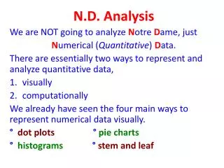
N.D. Analysis We are NOT going to analyze N otre D ame, just N umerical ( Quantitative ) D ata. There are essentially two ways to represent and analyze quantitative data, visually computationally We already have seen the four main ways to represent numerical data visually.

E N D
N.D. Analysis We are NOT going to analyze Notre Dame, just Numerical (Quantitative) Data. There are essentially two ways to represent and analyze quantitative data, • visually • computationally We already have seen the four main ways to represent numerical data visually. °dot plots °pie charts °histograms°stem and leaf
For the sake of completeness we look at an example of each: Dot Plot:
There is a fifth way, very inventive, called a box plot we will learn it a little later. We have to learn first how to work Computationally with a collection of numerical data. First of all we want to distinguish results computed from collections that come from a whole population from results computed from collections that come from a sample
Results from populations are called parameters • Results from samples are called statistics The rule is easy to remember: Population Parameter Sample Statistic (the PP-SS rule) With one exception, the calculations one does are the same, whether one is computing a parameter or a statistic. The exception will come later.
What kind of results will we be looking for? In other words, what calculations can you do on a given set of numbers? The list is endless, we have seen the following mentioned in class: Range, maximum, minimum, average, bidding method, variance, standard deviation, … A long standing convention stipulates that symbols used for parameters are Greek letters symbols used for statistics are latin letters A wonderful opportunity to learn some Greek letters! We will mostly use two: and
Important Calculations Time to start computing things. From now on, until stated otherwise, we assume we have a given set of numerical data x1, x2, x3,…, xn We also assume that we have already taken the trouble to order the data, that is x1 ≤ x2 ≤ x3 ≤ … ≤ xn We will be interested in “measuring” two concepts:
“Centrality” and “Spread” We measure “centrality” by trying to compute the “center” of the data. The trouble is that we don’t know what we mean by that’s right, the center ! Intuitively the center of two data, say 7 and 21, should be the midpoint, 14 (you don’t need your TI84 plus for this, I hope! ) But what if the data are 7, 7 and 21 ?
Most of you already know the answer …. That’s right, the average ! By the way, another word for average (more impressive!) is “mean”. Notation: The symbol for the sample mean is The symbol for the population mean is Using the notation we learned in the last class we can write: The mean has one serious defect:
It is extremely sensitive to extreme values. The following set of data 8 8 8 8 8 8 8 8 8 8 8 8 8 8 8 1,000,000 ought to have a center kind of close to 8 (there are 15 of them!) Instead your TI84 plus will tell you that the mean is 62,507.50(wow !) A more faithful (but harder to compute in general, and computationally less useful) measure of centrality is the median
You know the definition, essentially it is a number that cuts the ordered data into two equal halves. More precisely, If you have an odd number of data (think of 37), you pick the one smack in the middle (the 19-th, think about it!) If you have an even number of data (think of 46) you pick any number you please …. between the 23-rd and 24-th entries (if they are equal you got no choice!) We do a couple of examples on the board. Then one on the computer.
Distributional Symmetry(or lack thereof !) What’s the relationship, if any, between the median and the mean ?? Just for fun let’s call the median Md and the mean Mn (clever, huh ?). Then either Mn< Md or Mn = Md or Mn > Md Now, by its very definition Md is in the Middle! On the other hand, Mn is the average, the middlevalue. When the data are distributed in perfect symmetry we must therefore have Mn = Md What if Mn < Md? It means that somehow the average is pulled down to the left of the middle. There are more extreme values to the left. We say that the data are skewed to the left.
In the same way, if Mn> Md it means that somehow the average is pulled up to the right of the middle. There are more extreme values to the right. We say that the data are skewed to the right. Of course, there can’t be too many of these extreme values, on either side, because in that case the median is shifted. In terms of histograms, we get these four cases, shown on the next slides.
Distributions like the this one (symmetric and bunched around the middle) are said to be “nicely mound-shaped.” We’ll say more about them later.