Download
1 / 31
310 likes | 414 Vues
Study analyzing weather noise, feedback mechanisms, and ocean dynamics impacting North Atlantic SST variability from 1951-2000, implications for predictability using CGCM-class models and interactive ensembles.

E N D
Weather Noise Forcing of Low Frequency Variability in the North Atlantic Edwin K. Schneider COLA SAC Meeting April 2010
Collaborators • Meizhu Fan - many of the results come from her PhD thesis. • Ben Kirtman - developer of the “Interactive Ensemble” • David Straus • GMU Climate Dynamics Program students Hua Chen and Ioana Colfescu
Motivation • Diagnose and understand the mechanisms of observed low frequency observed (1951-2000) North Atlantic SST variability. • In particular, what were the roles of weather noise forcing, coupled feedbacks, and ocean dynamics? • What are the implications for “decadal” predictability?
Tripole Index: area averageSST difference (Czaja and Marshall 2001, QJRMS) 1951 2000
Approach • Simulate the observed 1951-2000 tripole index using a CGCM-class model forced by observed weather noise. • Try to understand the results in the framework of the simple model of Frankignoul and Hasselmann (1976) as extended by Marshall et al. (2001), Czaja and Marshall (2001): • Weather noise • Atmospheric feedback to SSTA • Gyre circulation • AMOC
Data and Models • NCEP reanalysis 1951-2000, monthly means • COLA CGCM • COLA V2 AGCM (T42, L18) • MOM3 OGCM (1.5º, finer meridional near equator) non-polar domain • Anomaly coupled • (RIP)
Mechanisms of Low Frequency Climate Variability (Sarachik et al., 1996) • Forced by atmospheric weather noise (Hasselmann 1976) • Forced by oceanic “weather noise” • Intrinsic coupled variability (e.g. coupled ocean-atmosphere) that is not forced by weather noise • Externally forced
Weather Noise • What is this “weather noise?” • Atmospheric motions that are NOT the response to the evolving surface boundary conditions (SST, etc.) or external forcing. • Unpredictable more than ~1 week in the future. • Properties of random (white) noise? • Determination of weather noise • Although unpredictable, it is straightforward to determine weather noise that has already occurred and been observed. • Subtract the atmospheric motions that ARE the response to the surface evolution (SST, etc.) or external forcing, as evaluated from an “AMIP ensemble,” from the total.
AMIP/GOGA Ensemble … Response 1 Response 2 Response N … AGCM AGCM AGCM 1 2 N EnsembleMean Response Observed time evolving SST, sea ice Response N = SST forced signal + NoiseN NoiseN is distinct for each N
… Response 1 Response 2 Response N … AGCM AGCM AGCM 1 2 N EnsembleMean Response (EMR) Observed time evolving SST, sea ice “OBS” Determination of Weather Noise Surface Fluxes Weather Noise =“OBS”- EMR
Example of Noise Evaluation: North Atlantic -NAO +NAO Anti-cyclonic over warm Cyclonic over cold Total Feedback Noise Opposite hf sign
What is the SST Response to Weather Noise? • Force a coupled model which has no internal weather noise with the “observed weather noise” surface fluxes as determined from the NCEP reanalysis. • Reproduce (or don’t reproduce) the observed SST evolution • Additional simulations to isolate the mechanisms responsible for the simulated SST evolution
Tool: Interactive Ensemble CGCM (IE CGCM; Kirtman et al.) • Couple an OGCM to a parameterized atmospheric model (as in an Intermediate Coupled Model). • The parameterized atmosphere is an AGCM ensemble. • The ocean sees the AGCM ensemble mean surface fluxes. • Each AGCM ensemble member sees the OGCM SST.
Interactive Ensemble CGCM … Response 1 Response 2 Response N … AGCM AGCM AGCM 1 2 N Ensemble Mean Surface Fluxes SST OGCM
Properties of IE CGCM • Atmospheric weather noise filtered out by ensemble mean • Internal SST variability is due to only ocean weather noise, coupled instability • Potentially much reduced low-frequency SST variability • Response of SST to a specified surface flux forcing (heat, wind stress, or fresh water) can be quasi-deterministic under some conditions • Includes full coupled feedbacks calculated from state-of-the-art parameterizations and a “perfect” transient eddy flux parameterization.
Response to Observed External Forcing 1870-2000 (20C3M) CCSM3 CMIP4 Colors = ensemble members Black= ensemble mean Red = CCSM3 ensemble mean Blue = CCSM3 IE
Experiments • Force Interactive Ensemble (IE) CGCM with weather noise surface fluxes for 1951-2000. • If the SST variability was the response to the weather noise, it will be reproduced. • Further experiments will then isolate the role of various processes in the SST variability (e.g. ocean dynamics, location and type of weather noise forcing, …) • Diagnostic only (“additive noise”).
Noise Forced Interactive Ensemble … Response 1 Response 2 Response N … AGCM AGCM AGCM 1 2 N Ensemble Mean Surface Fluxes SST Weather Noise Surface Fluxes OGCM
Other Ways to Think About Weather Noise Forced IE CGCM: • It is an OGCM simulation forced by observed fluxes but with feedbacks correctly taken into account. • “OGCM” simulations typically include atmospheric feedbacks (e.g. damping) as well as specified observed fluxes. This is inconsistent. • It is like a Coupled Data Assimilation
Understand Model Internal Variability • Perfect model, perfect data • The COLA CGCM NAO and tripole patterns are shifted eastward ~25° from the observed locations • The tripole is forced by weather noise heat fluxes • The mechanism was not fully diagnosed because of the large biases in the patterns • Perhaps we should revisit this, as understanding the cause of the biases may be central to interpreting the results concerning the observed tripole
Experiments to Diagnose Observed Variability • Forcing Data: 1951-2000 NCEP reanalysis monthly surface fluxes and SST Note: “all” ~ freshwater, heat, and momentum • N.B.: Bad model, inaccurate data, no external forcing in model or analysis
Tripole Index Observed NActl Gctl NAh
Tripole Index Observed NAm NActl Gctl NAh
The tripole index is locally forced by the weather noise heat flux (Gctl, NActl, NAh). • Momentum flux weather noise forces a tripole response that damps/lags the full response.
Extract model patterns by regression of simulation results against observed: tripole Index Observed NActl Gctl NAh NAm
Gyre Circulation and Variability in NActl Mean Gyre EOF 1 (31%) (“Intergyre Gyre”) PC1 of EOF1 (gyre index); NAO Index (observed)
Tripole and Gyre Indices NActl Gyre index: area avg. streamfn., 60°W-40°W, 35°-45°N
AMOC NActl NAh IE Unforced
COLA Model Diagnosis of the Observed North Atlantic SST Variability • The later 20th century North Atlantic tripole SST variability is predominantly forced by the local weather noise. • In the context of the simple model of Czaja and Marshall (2001), the observed tripole is in a damped, non-oscillatory regime, as opposed to a damped delayed oscillator regime. • So the decadal time scale (if there is one) is due to ?? • All hangs on the sign of the feedback between the atmospheric heat flux and SST (Palmer and Sun 1985) • Conjecture: biases in the stationary waves in the North Atlantic in the models (or in the blocked/unblocked regime transitions if the mean is the average of discrete regimes, e.g. Palmer et al. 2005) may be responsible for the perplexing results.
For Additional Details • Wu, Z., E. K. Schneider, and B. P. Kirtman, 2004: Causes of low frequency North Atlantic SST variability in a coupled GCM. Geophys. Res. Lett., 31, L09210, doi:10.1029/2004GL019548. • Schneider, E. K., 2006: Stochastic forcing of surface climate. COLA Technical Report 224, 34 pp. ftp://grads.iges.org/pub/ctr/ctr_224.pdf • Schneider, E. K. and M. Fan, 2007: Weather noise forcing of surface climate variability. J. Atmos. Sci., 64, 3265-3280. • Fan, M., 2009: Low frequency North Atlantic SST variability: Weather noise forcing and coupled response. PhD thesis, George Mason University. • Fan, M. and E. K. Schneider, 2010: Low frequency North Atlantic SST variability: Weather noise forcing and coupled response (in preparation).