Challenges in Atomic Force Microscopy: Overcoming Limitations for Enhanced Sensitivity
190 likes | 298 Vues
Atomic Force Microscopy (AFM) presents unique challenges including non-monotonic imaging signals, the influence of long-range and short-range forces, and significant noise, particularly 1/f noise in deflection sensors. Key factors affecting performance are thermal limits and measuring systems with high Q-factors. Identifying and optimizing laser power, along with methodologies such as frequency modulation detection and Tapping™ mode, can enhance sensitivity. This discussion highlights AFM's limitations, including sensor shot noise and the Heisenberg uncertainty principle.

Challenges in Atomic Force Microscopy: Overcoming Limitations for Enhanced Sensitivity
E N D
Presentation Transcript
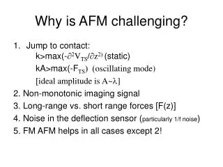
Why is AFM challenging? • Jump to contact: k>max(-¶2VTS/¶z2) (static) kA>max(-FTS) (oscillating mode) [ideal amplitude is A~l] 2. Non-monotonic imaging signal 3. Long-range vs. short range forces [F(z)] 4. Noise in the deflection sensor (particularly 1/f noise) 5. FM AFM helps in all cases except 2!
Thermal limits Energy in damped driven harmonic oscillator= kBT This allows one to determine the thermal limit of force gradient sensing in AFM: {zosc= F’ zo Q/k Is the signal near resonance}
Challenge of measuring high Q system Albrecht, Grutter, Horne Rugar J. Appl. Phys. 69, 668 (1994)
Better sensitivity with high Q cantilevers Q=115 slope detection Q=65,000 FM detection Q=65,000 slope detection Albrecht, Grutter, Horne Rugar J. Appl. Phys. 69, 668 (1994)
AC techniques Change in resonance curve can be detected by: • Lock-in (A or ) * • FM detection (f and Adrive) Albrecht, Grutter, Horne and Rugar J. Appl. Phys. 69, 668 (1991) (*) used in Tapping™ mode f A f1 f2 f3
Anczykowski et al., Appl. Phys. A 66, S885 (1998) Some words on Tapping™ Amount of energy dissipated into sample and tip stronglydepends on operation conditions. Challenging to determine magnitude or sign of force. NOT necessarily less power dissipation than repulsive contact AFM.
Ultimate limits of force sensitivity 1. Brownian motion of cantilever! thermal limits Martin, Williams, Wickramasinghe JAP 61, 4723 (1987) Albrecht, Grutter, Horne, and Rugar JAP 69, 668 (1991) D. Sarid ‘Scanning Force Microscopy’ T=4.5K A…rms amplitude A2 = kBT/k Roseman & Grutter, RSI 71, 3782 (2000) 2. Other limits: - sensor shot noise - sensor back action - Heisenberg D.P.E. Smith RSI 66, 3191 (1995) Bottom line: Under ambient conditions energy resolution ~ 10-24J << 10-21J/molecule
Other limitations? - sensor shot noise - sensor back action - Heisenberg D.P.E. Smith, Rev. Sci. Instr. 66, 3191 (1995)
Sensor Shot Noise Effectively, the fluctuations in laser pressure (due to photon statistics) give rise in a fluctuation in the mean position of the cantilever. P…laser power, Df…bandwidth l…wavelength h…Planck’s constant c…speed of light j…interferometer phase NB: can be used to ‘cool’ high finesse cavities!
Sensor Back Action Optical pressure Off resonance On resonance P…laser power, Df…bandwidth l…wavelength h…Planck’s constant c…speed of light
Optimization Minimize: and obtain optimized laser power (for off resonance set Q=1):
Heisenberg Minimal detectable energy with Minimal bandwidth Quantum limit
How about detecting a single spin? Idea: combine MFM and resonant excitation of the cantilever by combining ultimate AFM techniques and NMR.
MRFM D. Rugar, R. Budakian, H. J. Mamin & B. W. Chui, Nature 430, 329 (2004)
Another cool thing: thermodynamic squeezed state D. Rugar and P. Grutter, Phys. Rev. Lett. 67, 699 (1993)