Optimizing Index Access Scheduling for Top-k Queries in Document Retrieval Systems
370 likes | 489 Vues
This article presents an advanced methodology for index access scheduling in top-k document retrieval systems. It explores both Sorted Access (SA) and Random Access (RA) scheduling strategies aimed at maximizing the efficiency of document retrieval. The paper discusses the complexities involved in determining the optimal number of scan steps and investigates the trade-offs between performance costs across different access types. Key considerations for selectivity predictors, candidate document management, and effective scoring methods are also examined, culminating in a proposed combined algorithm that optimizes access based on expected scores and response times.

Optimizing Index Access Scheduling for Top-k Queries in Document Retrieval Systems
E N D
Presentation Transcript
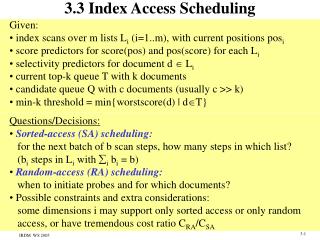
Given: • index scans over m lists Li (i=1..m), with current positions posi • score predictors for score(pos) and pos(score) for each Li • selectivity predictors for document d Li • current top-k queue T with k documents • candidate queue Q with c documents (usually c >> k) • min-k threshold = min{worstscore(d) | dT} 3.3 Index Access Scheduling • Questions/Decisions: • Sorted-access (SA) scheduling: • for the next batch of b scan steps, how many steps in which list? • (bi steps in Li with i bi = b) • Random-access (RA) scheduling: • when to initiate probes and for which documents? • Possible constraints and extra considerations: • some dimensions i may support only sorted access or only random • access, or have tremendous cost ratio CRA/CSA
Combined Algorithm (CA) assume cost ratio CRA/CSA = r perform NRA (TA-sorted) with [worstscore, bestscore] bookkeeping in priority queue Q and round-robin SA to m index lists ... after every r rounds of SA (i.e. m*r scan steps) perform RA to look up all missing scores of „best candidate“ in Q (where „best“ is in terms of bestscore, worstscore, or E[score], or P[score > min-k]) cost competitiveness w.r.t. „optimal schedule“ (scan until i highi≤ min{bestscore(d) | d final top-k}, then perform RAs for all d‘ with bestscore(d‘) > min-k): 4m + k
Sorted-Access Scheduling available info: L1 L2 L3 L4 Li 0.9 0.9 0.9 0.9 100 ... ... 100 100 100 0.8 0.9 0.9 0.8 200 score (posi) 200 200 200 posi 0.6 0.7 0.8 0.8 300 300 300 300 i 0.6 0.8 0.8 0.4 400 i 400 400 400 0.5 0.7 0.6 0.3 500 posi +bi 500 500 500 score (bi+ posi) 0.4 0.7 0.4 0.2 600 600 600 600 0.3 0.6 0.2 0.1 700 700 700 700 0.2 0.6 0.1 0.05 800 800 800 800 0.05 0.01 0.1 0.5 900 900 900 900 goal: eliminate candidates quickly aim for quick drop in highi bounds
SA Scheduling: Objective and Heuristics plan next b1, ..., bm index scan steps for batch of b steps overall s.t. i=1..m bi = b and benefit(b1, ..., bm) is max! possible benefit definitions: with score gradient with score reduction Solve knapsack-style NP-hard optimization problem (e.g. for batched scans) or use greedy heuristics: bi := b * benefit(bi=b) / =1..m benefit(b=b)
SA Scheduling: Benefit Aggregation Heuristics Consider current top-k T and andidate queue Q; for each d TQ we know E(d) 1..m, R(d) = 1..m – E(d), bestscore(d), worstscore(d), p(d) = P[score(d) > min-k] score current top-k candidates in Q bestscore(d) Sur- plus(d) with surplus(d) = bestscore(d) – min-k gap(d) = min-k – worstscore(d) i = E[score(j) | j [posi, posi+bi]] min-k gap(d) worstscore(d) weighs documents and dimensions in benefit function
Random-Access Scheduling: Heuristics Perform additional RAs when helpful 1) to increase min-k (increase worstscore of d top-k) or 2) to prune candidates (decrease bestscore of d Q) • For 1) Top Probing: • perform RAs for current top-k (whenever min-k changes), • and possibly for best d from Q • (in desc. order of bestscore, worstscore, or P[score(d)>min-k]) For 2) 2-Phase Probing: perform RAs for all candidates at point t total cost of remaining RAs = total cost of SAs up to t (motivated by linear increase of SA-cost(t) and sharply decreasing remaining-RA-cost(t))
Top-k Queries over Web Sources Typical example: Address = „2590 Broadway“ and Price = $ 25 and Rating = 30 issued against mapquest.com, nytoday.com, zagat.com Major complication: some sources do not allow sorted access highly varying SA and RA costs Major opportunity: sources can be accessed in parallel extension/generalization of TA distinguish S-sources, R-sources, SR-sources
Source-Type-Aware TA For each R-source Si Sm+1 .. Sm+r set highi := 1 Scan SR- or S-sources S1 .. Sm Choose SR- or S-source Si for next sorted access for object d retrieved from SR- or S-source Li do { E(d) := E(d) {i}; highi := si(q,d); bestscore(d) := aggr{x1, ..., xm) with xi := si(q,d) for iE(d), highi for i E(d); worstscore(d) := aggr{x1, ..., xm) with xi := si(q,d) for iE(d), 0 for i E(d); }; Choose SR- or R-source Si for next random access for object d retrieved from SR- or R-source Li do { E(d) := E(d) {i}; bestscore(d) := aggr{x1, ..., xm) with xi := si(q,d) for iE(d), highi for i E(d); worstscore(d) := aggr{x1, ..., xm) with xi := si(q,d) for iE(d), 0 for i E(d); }; current top-k := k docs with largest worstscore; min-k := minimum worstscore among current top-k; Stop when bestscore(d | d not in current top-k results) min-k ; Return current top-k; essentially NRA with choice of sources
Strategies for Choosing the Source for Next Access for next sorted acccess: Escore(Li) := expected si value for next sorted access to Li (e.g.: highi) rank(Li) := wi * Escore(Li) / cSA(Li) // wi is weight of Li in aggr // cSA(Li) is source-specific SA cost choose SR- or S-source with highest rank(Li) for next random acccess (probe): Escore(Li) := expected si value for next random access to Li (e.g.: (highi lowi) / 2) rank(Li) := wi * Escore(Li) / cRA(Li) choose SR- or R-source with highest rank(Li) or use more advanced statistical score estimators
The Upper Strategy for Choosing Next Object and Source (Marian et al.: TODS 2004) idea: eagerly prove that candidate objects cannot qualify for top-k for next random acccess: among all objects with E(d) and R(d) choose d‘ with the highest bestscore(d‘); if bestscore(d‘) < bestscore(v) for object v with E(v)= then perform sorted access next (i.e., don‘t probe d‘) else { := bestscore(d‘) min-k; if > 0 then { consider Li as „redundant“ for d‘ if for all Y R(d‘) {Li} jY wj * highj + wi * highi jY wj * highj ; choose „non-redundant“ source with highest rank(Li) } else choose source with lowest cRA(Li); };
The Parallel Strategy pUpper(Marian et al.: TODS 2004) idea: consider up to MPL(Li) parallel probes to the same R-source Li choose objects to be probed based on bestscore reduction and expected response time for next random acccess: probe-candidates := m objects d with E(d) and R(d) such that d is among the m highest values of bestscore(d); for each object d in probe-candidates do { := bestscore(d) min-k; if > 0 then { choose subset Y(d) R(d) such that jY wj * highj and expected response time LjY(d) ( |{d‘ | bestscore(d‘)>bestscore(d) and Y(d)Y(d‘)}| * cRA(Lj) / MPL(Lj) ) is minimum }; }; enqueue probe(d) to queue(Li) for all LiY(d) with expected response time as priority;
pTA: parallelized TA (with asynchronous probes, but same probe order as TA) Experimental Evaluation synthetic data real Web sources SR: superpages (Verizon yellow pages) R: subwaynavigator R: mapquest R: altavista R: zagat R: nytoday from: A. Marian et al., TODS 2004
3.4 Index Organization and Advanced Query Types • Richer Functionality: • Boolean combinations of search conditions • Search by word stems • Phrase queries and proximity queries • Wild-card queries • Fuzzy search with edit distance • Enhanced Performance: • Stopword elimination • Static index pruning • Duplicate elimination
Boolean Combinations of Search Conditions • combination of AND and ANDish: (t1 AND … AND tj) tj+1 tj+2… tm • TA family applicable with mandatory probing in AND lists • RA scheduling • (worstscore, bestscore) bookkeeping and pruning • more effective with “boosting weights” for AND lists combination of AND, ANDish and NOT: NOT terms considered k.o. criteria for results TA family applicable with mandatory probing for AND and NOT RA scheduling • combination of AND, OR, NOT in Boolean sense: • best processed by index lists in DocId order • construct operator tree and push selective operators down; • needs good query optimizer (selectivity estimation)
Search with Morphological Reduction (Lemmatization) • Reduction onto grammatical ground form: • nouns onto nominative, verbs onto infinitive, • plural onto singular, passive onto active, etc. • Examples (in German): • „Winden“ onto „Wind“, „Winde“ or „winden“ • depending on phrase structure and context • „finden“ and „gefundenes“ onto „finden“, • „Gefundenes“ onto „Fund“ • Reduction of morphological variations onto word stem: • flexions (e.g. declination), composition, verb-to-noun, etc. • Examples (in German): • „Flüssen“, „einflößen“ onto „Fluss“, • „finden“ and „Gefundenes“ onto „finden“ • „Du brachtest ... mit“ onto „mitbringen“, • „Schweinkram“, „Schweinshaxe“ and „Schweinebraten“ • onto „Schwein“ etc. • „Feinschmecker“ and „geschmacklos“ onto „schmecken“
Stemming • Approaches: • Lookup in comprehensive lexicon/dictionary (e.g. for German) • Heuristic affix removal (e.g. Porter stemmer for English): • remove prefixes and/or suffixes • based on (heuristic) rules • Example: • stresses stress, stressing stress, symbols symbol • based on rules: sses ss, ing , s , etc. The benefit of stemming for IR is debated. Example: Bill is operating a company. On his computer he runs the Linux operating system.
Phrase Queries and Proximity Queries phrase queries such as: „George W. Bush“, „President Bush“, „The Who“, „Evil Empire“, „PhD admission“, „FC Schalke 04“, „native American music“, „to be or not to be“, „The Lord of the Rings“, etc. etc. difficult to anticipate and index all (meaningful) phrases sources could be thesauri (e.g. WordNet) or query logs • standard approach: combine single-term index with separate position index term doc offset ... empire 39 191 empire 77 375 ... evil 12 45 evil 39 190 evil 39 194 evil 49 190 ... evil 77 190 ... term doc score ... empire 77 0.85 empire 39 0.82 ... evil 49 0.81 evil 39 0.78 evil 12 0.75 ... evil 77 0.12 ... B+ tree on term B+ tree on term, doc
Thesaurus as Phrase Dictionary Example: WordNet (Miller/Fellbaum), http://wordnet.princeton.edu
Biword and Phrase Indexing build index over all word pairs: index lists (term1, term2, doc, score) or for each term1 nested list (term2, doc, score) • variations: • treat nearest nouns as pairs, • or discount articles, prepositions, conjunctions • index phrases from query logs, compute correlation statistics • query processing: • decompose even-numbered phrases into biwords • decompose odd-numbered phrases into biwords • with low selectivity (as estimated by df(term1)) • may additionally use standard single-term index if necessary Examples: to be or not to be (to be) (or not) (to be) The Lord of the Rings (The Lord) (Lord of) (the Rings)
N-Gram Indexing and Wildcard Queries Queries with wildcards (simple regular expressions), to capture mis-spellings, name variations, etc. Examples: Brit*ney, Sm*th*, Go*zilla, Marko*, reali*ation, *raklion • Approach: • decompose words into N-grams of N successive letters • and index all N-grams as terms • query processing computes AND of N-gram matches • Example (N=3): • Brit*ney Bri AND rit AND ney Generalization: decompose words into frequent fragments (e.g., syllables, or fragments derived from mis-spelling statistics)
In addition to indexing all N-grams for some small N (e.g. 2 or 3), • determine frequent fragments – refstrings r R– with properties: • df(r) is above some threshold • if r R then for all substrings s of r: s R • unless df(s|r) = |{docs d | d contains s but not r}| Refstring Indexing (Schek 1978) • Refstring index build: • Candidate generation preliminary set R: • generate strings r with |r|>N in increasing length, compute df(r); • remove r from candidates if r=xy with df(x)< or df(y)< • Candidate selection: consider candidate r R with |r|=k and sets • left(r)={xr | xr R |xr|=k+1}, right(r)={ry | ry R |ry|=k+1}, • left(r)={xr | xr R |xr|=k+1}, right(r)={ry | R |ry|=k+1} • select r if weight(r) = df(r) – max{leftf(r), rightf(r)} with • leftf(r) = qleft(r) df(q) + qleft(r) max{leftf(q),rightf(q)} and • rightf(r) = qright(r) df(q) + qright(r) max{leftf(q),rightf(q)} QP decomposes term into small number of refstrings contained in t
Fuzzy Search with Edit Distance Idea: tolerate mis-spellings and other variations of search terms and score matches based on editing distance • Examples: • 1) query: Microsoft • fuzzy match: Migrosaft • score ~ edit distance 3 • query: Microsoft • fuzzy match: Microsiphon • score ~ edit distance 5 • 3) query: Microsoft Corporation, Redmond, WA • fuzzy match at token level: MS Corp., Redmond, USA
Similarity Measures on Strings (1) Hamming distance of strings s1, s2 * with |s1|=|s2|: number of different characters (cardinality of {i: s1i s2i}) Levenshtein distance (edit distance) of strings s1, s2 *: minimal number of editing operations on s1 (replacement, deletion, insertion of a character) to change s1 into s2 For edit (i, j): Levenshtein distance of s1[1..i] and s2[1..j] it holds: edit (0, 0) = 0, edit (i, 0) = i, edit (0, j) = j edit (i, j) = min { edit (i-1, j) + 1, edit (i, j-1) + 1, edit (i-1, j-1) + diff (i, j) } with diff (i, j) = 1 if s1i s2j, 0 otherwise efficient computation by dynamic programming
Similarity Measures on Strings (2) Damerau-Levenshtein distance of strings s1, s2 *: minimal number of replacement, insertion, deletion, or transposition operations (exchanging two adjacent characters) for changing s1 into s2 For edit (i, j): Damerau-Levenshtein distance of s1[1..i] and s2[1..j] : edit (0, 0) = 0, edit (i, 0) = i, edit (0, j) = j edit (i, j) = min { edit (i-1, j) + 1, edit (i, j-1) + 1, edit (i-1, j-1) + diff (i, j), edit (i-2, j-2) + diff(i-1, j) + diff(i, j-1) +1 } with diff (i, j) = 1 if s1i s2j, 0 otherwise
Similarity based on N-Grams Determine for string s the set of its N-Grams: G(s) = {substrings of s with length N} (often trigrams are used, i.e. N=3) Distance of strings s1 and s2: |G(s1)| + |G(s2)| - 2|G(s1)G(s2)| Example: G(rodney) = {rod, odn, dne, ney} G(rhodnee) = {rho, hod, odn, dne, nee} distance (rodney, rhodnee) = 4 + 5 – 2*2 = 5 Alternative similarity measures: Jaccard coefficient: |G(s1)G(s2)| / |G(s1)G(s2)| Dice coefficient: 2 |G(s1)G(s2)| / (|G(s1)| + |G(s2)|)
N-Gram Indexing for Fuzzy Search Theorem (Jokinen and Ukkonen 1991): for query string s and a target string t, the Levenshtein edit distance is bounded by the N-Gram overlap: • for fuzzy-match queries with edit-distance tolerance d, perform top-k query over Ngrams, using count for score aggregation
Phonetic Similarity (1) • Soundex code: • Mapping of words (especially last names) onto 4-letter codes • such that words that are similarly pronounced have the same code • first position of code = first letter of word • code positions 2, 3, 4 (a, e, i, o, u, y, h, w are generally ignored): • b, p, f, v 1 c, s, g, j, k, q, x, z 2 • d, t 3 l 4 • m, n 5 r 6 • Successive identical code letters are combined into one letter • (unless separated by the letter h) Examples: Powers P620 , Perez P620 Penny P500, Penee P500 Tymczak T522, Tanshik T522
Phonetic Similarity (2) Editex similarity: edit distance with consideration of phonetic codes For editex (i, j): Editex distance of s1[1..i] and s2[1..j] it holds: editex (0, 0) = 0, editex (i, 0) = editex (i-1, 0) + d(s1[i-1], s1[i]), editex (0, j) = editex (0, j-1) + d(s2[j-1], s2[j]), editex (i, j) = min { editex (i-1, j) + d(s1[i-1], s1[i]), editex (i, j-1) + d(s2[j-1], s2[j]), edit (i-1, j-1) + diffcode (i, j) } with diffcode (i, j) = 0 if s1i= s2j, 1 if group(s1i)= group(s2j), 2 otherwise und d(X, Y) = 1 if X Y and X is h or w, diffcode (X, Y) otherwise with group: {a e i o u y}, {b p}, {c k q}, {d t}, {l r}, {m n}, {g j}, {f p v}, {s x z}, {c s z}
3.4 Index Organization and Advanced Query Types • Richer Functionality: • Boolean combinations of search conditions • Search by word stems • Phrase queries and proximity queries • Wild-card queries • Fuzzy search with edit distance • Enhanced Performance: • Stopword elimination • Static index pruning • Duplicate elimination
Stopword Elimination Lookup in stopword list (possibly considering domain-specific vocabulary, e.g. „definition“ or „theorem“ in math corpus Typical English stopwords (articles, prepositions, conjunctions, pronouns, „overloaded“ verbs, etc.): a, also, an, and, as, at, be, but, by, can, could, do, for, from, go, have, he, her, here, his, how, I, if, in, into, it, its, my, of, on, or, our, say, she, that, the, their, there, therefore, they, this, these, those, through, to, until, we, what, when, where, which, while, who, with, would, you, your
Static Index Pruning (Carmel et al. 2001) Scoring function S‘ is an -variation of scoring function S if (1)S(d) ≤ S‘(d) ≤ (1+)S(d) for all d Scoring function Sq‘ for query q is (k, )-good for Sq if there is an -variation S‘ of Sq such that the top-k results for Sq‘ are the same as those for S‘. Sq‘ for query q is (, )-good for Sq if there is an -variation S‘ of Sq such that the top- results for Sq‘ are the same as those for S‘, where top- results are all docs with score above *score(top-1) Given k and , prune index lists so as to guarantee (k, r)-good results for all queries q with r terms where r < 1/ . for each index list Li, let si(k) be the rank-k score; prune all Li entries with score < * si(k)
Efficiency and Effectiveness of Static Index Pruning from: D. Carmel et al., Static Index Pruning for Information Retrieval Systems, SIGIR 2001
Duplicate Elimination (Broder 1997) duplicates on the Web may be slightly perturbed crawler & indexing interested in identifying near-duplicates • Approach: • represent each document d as set (or sequence) of • shingles (N-grams over tokens) • encode shingles by hash fingerprints (e.g., using SHA-1), • yielding set of numbers S(d) [1..n] with, e.g., n=264 • compare two docs d, d‘ that are suspected to be duplicates by • resemblance: • containment: • drop d‘ if resemblance or containment is above threshold
MIPs (set1) MIPs (set2) 8 8 8 9 9 24 N 33 45 … 24 24 9 36 48 9 13 MIPs vector: minima of perm. estimated resemblance = 2/6 set of ids Min-Wise Independent Permutations (MIPs) 17 21 3 12 24 8 h1(x) = 7x + 3 mod 51 20 48 24 36 18 8 h2(x) = 5x + 6 mod 51 40 9 21 15 24 46 … hN(x) = 3x + 9 mod 51 9 21 18 45 30 33 compute N random permutations with: P[min{(x)|xS}=(x)] =1/|S| MIPs are unbiased estimator of resemblance: P [min {h(x) | xA} = min {h(y) | yB}] = |AB| / |AB| MIPs can be viewed as repeated sampling of x, y from A, B
Efficient Duplicate Detection in Large Corpora avoid comparing all pairs of docs • Solution: • for each doc compute shingle-set and MIPs • produce (shingleID, docID) sorted list • produce (docID1, docID2, shingleCount) table • with counters for common shingles • Identify (docID1, docID2) pairs • with shingleCount above threshold • and add (docID1, docID2) edge to graph • Compute connected components of graph (union-find) • these are the near-duplicate clusters • Trick for additional speedup of steps 2 and 3: • compute super-shingles (meta sketches) for shingles of each doc • docs with many common shingles have common super-shingle w.h.p.
Top-k Query Processing: • Grossman/Frieder Chapter 5 • Witten/Moffat/Bell, Chapters 3-4 • A. Moffat, J. Zobel: Self-Indexing Inverted Files for Fast Text Retrieval, • TOIS 14(4), 1996 • R. Fagin, A. Lotem, M. Naor: Optimal Aggregation Algorithms for Middleware, • J. of Computer and System Sciences 66, 2003 • S. Nepal, M.V. Ramakrishna: Query Processing Issues in Image (Multimedia) • Databases, ICDE 1999 • U. Guentzer, W.-T. Balke, W. Kiessling: Optimizing Multi-FeatureQueries in • Image Databases, VLDB 2000 • C. Buckley, A.F. Lewit: Optimization of Inverted Vector Searches, SIGIR 1985 • M. Theobald, G. Weikum, R. Schenkel: Top-k Query Processing with • Probabilistic Guarantees, VLDB 2004 • M. Theobald, R. Schenkel, G. Weikum: Efficient and Self-Tuning • Incremental Query Expansion for Top-k Query Processing, SIGIR 2005 • X. Long, T. Suel: Optimized Query Execution in Large Search • Engines with Global Page Ordering, VLDB 2003 • A. Marian, N. Bruno, L. Gravano: Evaluating Top-k Queries over • Web-Accessible Databases, TODS 29(2), 2004 Additional Literature for Chapter 3
Additional Literature for Chapter 3 • Index Organization and Advanced Query Types: • Manning/Raghavan/Schütze, Chapters 2-6, http://informationretrieval.org/ • H.E. Williams, J. Zobel, D. Bahle: Fast Phrase Querying with Combined Indexes, • ACM TOIS 22(4), 2004 • WordNet: Lexical Database for the English Language, http://wordnet.princeton.edu/ • H.-J. Schek: The Reference String Indexing Method, ECI 1978 • D. Carmel, D. Cohen, R. Fagin, E. Farchi, M. Herscovici, Y.S. Maarek, A. Soffer: • Static Index Pruning for Information Retrieval Systems, SIGIR 2001 • G. Navarro: A guided tour to approximate string matching, • ACM Computing Surveys 33(1), 2001 • G. Navarro, R. Baeza-Yates, E. Sutinen, J. Tarhio: Indexing Methods for • Approximate String Matching. IEEE Data Engineering Bulletin 24(4), 2001 • A.Z. Broder: On the Resemblance and Containment of Documents, • Compression and Complexity of Sequences Conference 1997 • A.Z. Broder, M. Charikar, A.M. Frieze, M. Mitzenmacher: Min-Wise • Independent Permutations, Journal of Computer and System Sciences 60, 2000