by Symon Kimitei Spring ‘2005
570 likes | 807 Vues
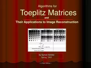
Algorithms for Toeplitz Matrices. and. Their Applications to Image Reconstruction. by Symon Kimitei Spring ‘2005. O(nlog 2 n) Superfast Linear Least Squares Schur Algorithm. Abstract.

by Symon Kimitei Spring ‘2005
E N D
Presentation Transcript
Algorithms for Toeplitz Matrices and Their Applications to Image Reconstruction by Symon Kimitei Spring ‘2005 ~ A Thesis Defense ~
O(nlog2n) Superfast Linear Least Squares Schur Algorithm Abstract • This algorithm illustrates another way of solving linear equations or linear least squares problems with low displacement rank. • The algorithm we present is based on the fast O(n2) Schur algorithm but speeded up computationally via the FFT • In particular, we examine regularized least squares problems with displacement rank 4 • Such low displacement rank problems indicates that solutions to them can be found easily by Cholesky factorization methodwhich decomposes any positive symmetric definite matrix intoCTC where C is the Cholesky factor and is upper triangular • Instructively, the system we solve has a Toeplitz-like structure which can be exploited algorithmically and can model image blurring and deblurring procedures SlowFastSuperFast ~ A Thesis Defense ~ A Synopsis of Algorithms
Outline • SECTION 1: Introduction and other background information • SECTION 2: The Generalized Schur Algorithm • SECTION 3: The Superfast Least Squares Schur Algorithm • SECTION 4: Complexity and Storage Analysis • SECTION 5: Application of algorithms to Image deblurring • SECTION 6: Results and Analysis • SECTION 7: Conclusion • (References) ~ A Thesis Defense ~
There are four areas of D.I.P: Image Restoration, Enhancement, Compression, Recognition • Our Thesis project examines the problem of Image restoration • Image restoration deals with cleaning degraded images using mathematical procedures • A degraded image implies that it has noise in it • Sources of image degradation include: • Camera out-of-focus • Environmental degradation [like poorly stored family snaps] • Relative camera-object motion • Sensor noise during image capture • Atmospheric turbulence as in military reconnaissance planes Introduction ~ A Thesis Defense ~
The blurred image representation: Original Image Intro…Blurred ImageRepresentation B=T1 X T2 + F RandomizedNoise Blurred Image • In D.I.P, an image is represented by a2-D signal – An array of matrix coefficients Toeplitz ~ A Thesis Defense ~ Derivation…
In solving for X, since T1 and T2 are ill-conditioned, it is not sufficientto compute: Intro…Magnified Errors • Image Error becomes: • Instead we compute X to be: ~ A Thesis Defense ~
Tikhonov Regularization • We use Tikhonov regularization technique in our Thesis to damp out errors in the linear least squares problem we are solving. • The technique allows us to stabilize the solutions for the problem with the use of a regularization operator. • Such that given: • Then we solve the regularized system which requires that we compute the minimization: • We set Y=XT2. ~ A Thesis Defense ~
Continued… • Solving for: Tikhonov Regularization • This allows for the formulation of another least squares problem: • Where the regularization parameter ≥0. • This means we can compute for: • Whose normal equations are: Derivation… ~ A Thesis Defense ~
In order to decompose the matrix being solved into upper and lower triangular form in our algorithms in this Thesis, we will need to introduce zeros to a matrix or a vector appropriately. Hyperbolic Rotations • To do so, we use Hyperbolic rotations which is a matrix of the form: • Hyperbolic rotations satisfy the relation: ~ A Thesis Defense ~
Continued… • As an example, suppose we apply hyperbolic rotations to the matrix. Hyperbolic Rotations • Our goal is to use hyperbolic rotations to insert a zero at location of the element g21 • Setting ~ A Thesis Defense ~
The Image Deblurring Algorithms • There are four algorithms to discuss which form the basis of image restoration using a Toeplitz-like matrix They are: The generalized Schur Algorithm (gschur) The Super Fast Least Squares Schur Algorithm (sflsschur) ~ A Thesis Defense ~
The Generalized Schur Algorithm • This algorithm is used to factorize a Toeplitz-like matrix of low displacement rank. • It is a popular fast method for the Cholesky factorization of a symmetric, positive definite Toeplitz matrix. • The fact that the Toeplitz-like matrix is s.p.d implies that it can be decomposed by the Cholesky factorization process into: • Where Cis upper triangular. • So by back substitution we can compute the Cholesky factors within a runtime of: O(n2) ~ A Thesis Defense ~
The Generalized Schur Algorithm Cholesky Factorization Zero-borderedSchurComplement • Given a symmetric, positive definite Toeplitz matrix: • By the Cholesky factorization procedure FirstCholesky row ~ A Thesis Defense ~
The Generalized Schur Algorithm Cholesky Factorization Zero-borderedSchurComplement First Cholesky row • If we zero the first column of the Schur complement, the result is the second Cholesky row. • The procedure is done recursively to reveal all of the Cholesky rows so that we can define: T=CTC ~ A Thesis Defense ~
The Generalized Schur Algorithm Continued… • Therefore, given a rectangular Toeplitz matrix, such that: • We can find a reduced representation of TT T. ~ A Thesis Defense ~
The Generalized Schur Algorithm Continued... • We will use a displacement equation defined as • Where G is the generator matrix. • The downshift matrix Z is defined as: • The signature matrix, ∑ , is defined as: ~ A Thesis Defense ~
The Generalized Schur Algorithm Continued… • Now given T, we can easily partition it so that: ~ A Thesis Defense ~ Derivation…
The Generalized Schur Algorithm Continued… • Definition of the Generator matrix G: Derivation… ~ A Thesis Defense ~
The Generalized Schur Algorithm Continued… • In general we work with any matrix M=TTT+2Isuch that • Where the ∑-Orthogonal matrix is a matrix H such that H∑HT=∑where ~ A Thesis Defense ~
Contd. The Generalized Schur Algorithm • We can use hyperbolic and plane rotations to zero the elements of GT to yield: which is in proper form ~ A Thesis Defense ~
Continued... The Generalized Schur Algorithm • So when • In general we will always choose H to put GTin proper form. ~ A Thesis Defense ~
The Generalized Schur Algorithm Continued... • Lets also define the first row of M to be: • Without regularization • This means that we denote Where • Using the displacement equation definition, it is easy to see that ~ A Thesis Defense ~
The Generalized Schur Algorithm Contd. The idea is to reduce the polynomials to proper form • In general, given the Generator Matrix, the following steps are undertaken: • Apply the downshift matrix on:: Scalars Vectors of dimension n-1X1 • Where the downshift matrix is given by • Apply hyperbolic and plane rotations on the generator matrix to yield • The result is the generator matrix for the Schur complement • The first Cholesky row becomes • Applying the same procedures to the Schur complement yields the 2nd Cholesky row. Go recursively to yield subsequent Cholesky rows ~ A Thesis Defense ~
Continued… The Generalized Schur Algorithm Clearly, • Where Gs contains the proper form generators for Ms • This means that zero-bordered Ms inherits the displacement structure of M • Alongside, the generators of Ms are determined by the proper form generators of TTT • The process is done recursively on Ms with the generators Gsto successively compute the subsequent rows of the Cholesky factor ~ A Thesis Defense ~
The Super Fast Least Squares Schur Algorithm Contd. • If instead we let M=TTT+2I and apply the displacement operator it is easy to see that: Displacement rank 5 Reduced to displacement rank 4 ~ A Thesis Defense ~
The Super Fast Least Squares Schur Algorithm Contd. • Therefore a more explicit definition for the generator matrix is: • Generator definition as column vectors • Generator definition as polynomials ~ A Thesis Defense ~
The Super Fast Least Squares Schur Algorithm Contd. The idea is to reduce the polynomials to proper form • Steps of the algorithm to yield step 1 polynomials • If we iterate, it means that the following result yields step k polynomials ~ A Thesis Defense ~
The Super Fast Least Squares Schur Algorithm Contd. The idea is to reduce the polynomials to proper form • In general, given the Generator Matrix, the following steps are undertaken: Matrix Generator of dimension 1X4 • Apply hyperbolic and plane rotations on the generator matrix to yield ~ A Thesis Defense ~
The Super Fast Least Squares Schur Algorithm Contd. The idea is to reduce the polynomials to proper form • In general, given the Generator Matrix, the following steps are undertaken: • The first Cholesky row becomes • Apply the downshift matrix on:: ~ A Thesis Defense ~
The Super Fast Least Squares Schur Algorithm Contd. The idea is to reduce the polynomials to proper form The downshift operation: ~ A Thesis Defense ~
The Super Fast Least Squares Schur Algorithm Contd. The idea is to reduce the polynomials to proper form • Having reduced the polynomials to proper form, the algorithm is reformulated to use matrix-vector multiplication which has computation speed up via the FFT • We start with the partitioning: • The partitioning is such that one can take advantage of the divide and conquer technique. ~ A Thesis Defense ~
The Super Fast Least Squares Schur Algorithm Contd. • Given the partitioning, the transformations that perform k-steps of the Super fast least squares Schur algorithm is defined Generators at the initial stage Generators at the k-step Downshifting matrix Hyperbolic & Plane rotations ~ A Thesis Defense ~
The Super Fast Least Squares Schur Algorithm Contd. • The same result can be obtained by the operation ~ A Thesis Defense ~
The Super Fast Least Squares Schur Algorithm Contd. Evaluates the generators of the Schur complement: Continues the Factorization on the Schur complement Ms : Combines the firs n/2 stepswith the last n/2 steps ~ A Thesis Defense ~
The Super Fast Least Squares Schur Algorithm Contd. Computing the Generators of M-1 • Then by the displacement equation definition Given Where • It is clear to see that has the Schur complement Derivation… ~ A Thesis Defense ~
The Super Fast Least Squares Schur Algorithm Contd. Computing the Generators of M-1 • But if we let Then: • Recall from earlier that: ~ A Thesis Defense ~
The Super Fast Least Squares Schur Algorithm Contd. Computing the Generators of M-1 • Which can further be expressed as: • From the displacement equation of the Augmented matrix we can see that: ~ A Thesis Defense ~
The Super Fast Least Squares Schur Algorithm Contd. Computing the Generators of M-1 • More generally, the displacement of M can be expressed as ~ A Thesis Defense ~ Derivation…
The Super Fast Least Squares Schur Algorithm Contd. Computing the Generators of M-1 ~ A Thesis Defense ~
The Super Fast Least Squares Schur Algorithm Contd. Computing the Generators of M-1 • More generally, the matrix M can be expressed as • Where A, B, C, D are lower triangular Toeplitz matrices and are also the generators of M • This fact is a generalization of the Gohberg-Semencul formula for the inverse of a Toeplitz matrix • Since the matrices A, B, C, D can be embedded in a 2n X 2n Circulant matrix, we can do fast multiplication by M-1via the FFT which gives computational speedup ~ A Thesis Defense ~ Derivation…
The Super Fast Least Squares Schur Algorithm Contd. Computing the Generators of M-1 • If H(z) does n steps of the superfast linear least squares Schur algorithm on the generators of M-1given by • It implies that after n steps of the algorithm, we will have the generators of the augmented matrix ~ A Thesis Defense ~
The Super Fast Least Squares Schur Algorithm Contd. Computing the Generators of M-1 • To calculate the polynomial generators, the following relations • The relations computes the generators of M-1 ~ A Thesis Defense ~
The Super Fast Least Squares Schur Algorithm Contd. Fast multiplication of M-1 via the FFT • Fast matrix-vector multiplication with a Toeplitz matrix can be performed at time complexity of O(nlogn). • This process works by embedding a n X n Toeplitz matrix into a large 2n X 2n circulant matrix C so that the vectors are padded with zeros ~ A Thesis Defense ~
The Super Fast Least Squares Schur Algorithm Contd. Fast multiplication of M-1 via the FFT • Note that each column of the circulant matrix is obtained by doing a downshift wraparound of the previous column • A circulant matrix is defined as • More explicitly, the elements are defined as: ~ A Thesis Defense ~
The Super Fast Least Squares Schur Algorithm Contd. • The resulting Circulant matrix is: Fast Multiplication via FFT • Given a Toeplitz matrix • We can generate the first column of the Circulant matrix as ~ A Thesis Defense ~
The Super Fast Least Squares Schur Algorithm Contd. Fast Multiplication via the FFT • To evaluate y=Tx,we set • So we can obtain y as the topn elements in the product • General Steps ~ A Thesis Defense ~
Complexity & Storage Analysis Contd. Storage Analysis It can be shown that the solution to the recurrence is: ~ A Thesis Defense ~
Complexity & Storage Analysis Contd. Computational Speed Analysis It can be shown that this Superfast Least Squares Schur algorithm satisfies the recurrence: Hence, Thus our Superfast linear least squares Schur algorithm has a computational complexity ofO(nlog2n) ~ A Thesis Defense ~
Measuring The Image Deblurring Results • The Mean-Squared Error • The Relative Error • The Peak Signal-to-Noise Ratio Where S is the maximum pixel value. PSNR is measure in decibel (db) ~ A Thesis Defense ~
Contd. Image Deblurring results I ~ A Thesis Defense ~