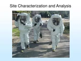
Site Characterization Using Physical and Chemical Methodologies
This workshop presented by Kent Novakowski at Queens University outlines methodologies for characterizing fractured bedrock and understanding groundwater transport dynamics. Key topics included the complexity of discrete fracture pathways, the challenges of measuring hydraulic properties, and the limitations of traditional methods like Darcy's Law. It emphasized the importance of detailed hydraulic testing and the use of cubic law for estimating groundwater velocities. The session also discussed the role of fractures' inter-connectivity and matrix diffusion, along with practical modeling techniques for improved prediction of groundwater flows.

Site Characterization Using Physical and Chemical Methodologies
E N D
Presentation Transcript
Site Characterization Using Physical and Chemical Methodologies Kent Novakowski Queens University Kingston, ON EPA Fractured Bedrock Workshop
Conceptual Model Development • Transport through discrete fracture pathways • Pathway inter-connectivity • Groundwater velocity • Matrix diffusion • Vertical fractures • Modeling
Discrete Fractures • Very difficult to obtain hydraulic properties of specific fractures • Geophysics is of limited use • Measure hydraulics directly using an interval testing method • Mean fracture spacing and scale play a significant role
Groundwater Velocity • Proportional to the square of the fracture aperture (cubic law) • Darcy’s Law does not work • Must know discrete fracture properties to predict velocity
Example Four Fractures, 6-m interval T=4x10⁻⁵ m2/s
Example • Estimate velocity via Darcy’s Law using T, i=0.001 and assuming a porosity of 1% = 0.06 m/day • Equivalent single fracture aperture is 410 μm, thus velocity calculated using cubic law = 8.5 m/day
Example • Assume fractures contribute evenly, aperture of each is then 257 μm • Using the cubic law, the true velocity in each fracture is 3.4 m/day • Detailed hydraulic testing results help this calculation immensely
Groundwater Velocity • Measurement of hydraulic gradient another difficulty with velocity calculations • Gradient often limited by “critical neck” at the network scale • May be safest to use estimate of regional gradient and not direct measurement
Hydraulic Head • Very powerful information from which to infer connectivity • Need hydraulic head over entire borehole (not just a discrete zone) • Requires multi-level completions – the more discrete intervals the better
Example Isolate intervals using packer elements Measure hydraulic head in each interval
40 m borehole 8 isolated intervals 82% of borehole accessible
Interpretation of Hydraulic Head • Two laterally-continuous flat lying fractures separated by 0.8 m vertically • Difference in hydraulic head between the two fractures of 2.0 m • Two boreholes 15 m apart
APERTURE (μm) Borehole Upper Fracture Lower Fracture 1 135 <10 2 <10 210 • Presumed hydraulic gradient = 0.13 • Real hydraulic gradient = 0.0015
Modeling • Once the discrete pathways are discovered, use a pathway model that accurately simulates the transport processes • Analytical models can be easily used for this • Choose an appropriate aperture and fracture spacing
Conclusions • Major discrete fracture pathways must be identified • Use hydraulic head to determine inter-connectivity • Estimate groundwater velocity using cubic law • Use angle drilling to identify vertical fractures • Simple pathway modeling (including matrix diffusion) very powerful tool