Household Behavior and Consumer Choice
390 likes | 415 Vues
Household Behavior and Consumer Choice. Appendix: Indifference Curves. Prepared by: Fernando Quijano and Yvonn Quijano. Understanding the Microeconomy and the Role of Government. Firm and Household Decisions.

Household Behavior and Consumer Choice
E N D
Presentation Transcript
Household Behaviorand Consumer Choice Appendix: Indifference Curves Prepared by: Fernando Quijano and Yvonn Quijano
Firm and Household Decisions • Households demand in output markets and supply labor and capital in input markets.
Assumptions • A key assumption in the study of household and firm behavior is that all input and output markets are perfectly competitive. • Perfect competition is an industry structure in which there are many firms, each small relative to the industry, producing virtually identical (or homogeneous) products and in which no firm is large enough to have any control over price.
Assumptions • We also assume that households and firms possess all the information they need to make market choices. • Perfect knowledge is the assumption that households posses a knowledge of the qualities and prices of everything available in the market, and that firms have all available information concerning wage rates, capital costs, and output prices.
Household Choice in Output Markets • Every household must make three basic decisions: • How much of each product, or output, to demand. • How much labor to supply. • How much to spend today and how much to save for the future.
The Determinants of Household Demand (as seen in Chapter 3) Factors that influence the quantity of a given good or service demanded by a single household include: • The price of the product in question. • The income available to the household. • The household’s amount of accumulated wealth. • The prices of related products available to the household. • The household’s tastes and preferences. • The household’s expectations about future income, wealth, and prices.
The Budget Constraint • The budget constraint refers to the limits imposed on household choices by income, wealth, and product prices. • A choice set or opportunity set is the set of options that is defined by a budget constraint.
The Budget Constraint • A budget constraint separates those combinations of goods and services that are available, given limited income, from those that are not. • The available combinations make up the opportunity set.
The Budget Constraint • The real cost of a good or service is its opportunity cost, and opportunity cost is determined by relative prices.
This is the budget constraint when income equals $200 dollars per month, the price of jazz club visits is $10 each, and the price of a Thai meal is $20. The Budget Constraint • One of the possible combinations is 5 Thai meals and 10 Jazz club visits per month.
Point E is unattainable given the current income prices. Point D does not exhaust the entire income available. The Budget Constraint
The Budget Constraint • A decrease in the price of Thai meals shifts the budget line outward along the horizontal axis. • The decrease in the price of one good expands the consumer’s opportunity set.
The Basis of Choice: Utility • Utility is the satisfaction, or reward, a product yields relative to its alternatives. The basis of choice. • Marginal utility is the additional satisfaction gained by the consumption or use of one more unit of something.
Diminishing Marginal Utility • The law of diminishing marginal utility: The more of one good consumed in a given period, the less satisfaction (utility) generated by consuming each additional (marginal) unit of the same good.
Diminishing Marginal Utility • Total utility increases at a decreasing rate, while marginal utility decreases.
Allocating Income to Maximize Utility Ice Cream P=$2 Pizza P=$1 Quantity Total Util. Marginal Util. Total Util. Marginal Util.
Allocating Income to Maximize Utility • The pizzais $1 a slice and the Ice Cream is $2 a scoop. I have $7 in my pocket. I want to choose the combination of pizza and Ice Cream that gives me the greatest possible utility for my $7. • I bought 3 slices of pizza which give a total utility of 56 and 2 scoops of ice cream which give a total utility of 44. My total utility from lunch is 56+44=100. There is no other combination of pizza and ice cream that give a greater utility for $7.
Allocating Income to Maximize Utility • In order to maximize utility, an individual is to choose the items lying within his budget constraint that gives him the most utility per dollar spent. • The consumer should therefore purchase all goods up to the quantities at which the marginal utility per dollar is equal for all the goods. That is the utility maximizing rule.
Income and Substitution Effects • The income effect: Consumption changes because purchasing power changes. • The substitution effect: Consumption changes because opportunity costs change. Price changes affect households in two ways:
Income and Substitution Effectsof a Price Change (for normal goods) Income effect: • When the price of a product falls, a consumer has more purchasing power with the same amount of income. • When the price of a product rises, a consumer has less purchasing power with the same amount of income. • Substitution effect: • When the price of a product falls, that product becomes more attractive relative to potential substitutes. • When the price of a product rises, that product becomes less attractive relative to potential substitutes.
Income and Substitution Effectsof a Price Change (for normal goods)
Consumer Surplus • Consumer surplus is the difference between the maximum amount a person is willing to pay for a good and its current market price. • The demand curve is a representation of what people are willing to pay at a given quantity. Therefore, the difference between the price and the demand curve is the consumer surplus for a given quantity.
Consumer Surplus P S $9 Consumer Surplus for the first case of soda is $ 9 - $ 5 = $ 4, for the second case is $ 7 - $ 5 = $ 2, and For the third one is $ 5 - $ 5 = $ 0. $7 $5 D 0 Q 3 1 2
Consumer Surplus The area of this triangle is the total Consumer Surplus P S This is the generally accepted method of finding the total Consumer Surplus in a market P* D 0 Q Q*
Household Choice in Input Markets • Whether to work • How much to work • What kind of a job to work at As in output markets, households face constrained choices in input markets. They must decide: • These decisions are affected by: • The availability of jobs • Market wage rates • The skill possessed by the household
The Price of Leisure • The wage rate can be thought of as the price—or the opportunity cost– of the benefits of either unpaid work or leisure. • The decision to enter the workforce involves a trade-off between wages on the one hand, and leisure and the value of nonmarket production on the other.
The Labor Supply Curve • The labor supply curve is a diagram that shows the quantity of labor supplied at different wage rates.
Income and SubstitutionEffects of a Wage Change • An increase in the wage rate affects households in two ways, known as the substitution and income effects. • The substitution effect of a higher wage means that the opportunity cost of leisure is higher. Each hour of leisure at a higher wage costs more.The household will buy less leisure (supply more labor). • When the substitution effect outweighs the income effect, the labor supply curve slopes upward.
Income and SubstitutionEffects of a Wage Change • An increase in the wage rate affects households in two ways, known as the substitution and income effects. • The income effect of a higher wage means that households can afford to buy more leisure (offer less labor). • When the income effect outweighs the substitution effect, the result is a “backward-bending” labor supply curve.
Saving and Borrowing:Present Versus Future Consumption • Households can use present income to finance future spending (i.e., save), or they can use future funds to finance present spending (i.e., borrow). • In deciding how much to save and how much to spend today, interest rates define the opportunity cost of present consumption in terms of foregone future consumption.
Appendix: Indifference Curves • An indifference curve shows bundles of goods that make the consumer equally happy. • The consumer is indifferentat points A, B, and C because they are all on the same curve. • The consumer is worse off at A’ than at A.
Appendix: Indifference Curves • A preference map is a whole set of indifference curves. • Higher indifference curves represent larger quantities of goods than do lower indifference curves. Therefore, higher indifference curves are preferred to lower ones. • Here i4 yields the highest total utility among the four indifference curves.
Appendix: Indifference Curves • The indifference curves are convex toward the origin. • The marginal rate of substitution(MRS)is the amount of one product that a consumer is willing to give up to get one more unit of another product. • MRS is the slope at any point on an indifference curve and it is defined as MUX \ MUY. • MRS is negative.
Quantity of Pepsi 14 MRS = 6 A 8 1 4 B MRS = 1 3 Indifference 1 curve 2 3 6 7 Quantity of Pizza Appendix: Indifference Curves • People are more willing to trade away goods that they have in abundance and less willing to trade away goods of which they have little. This illustrates the hypothesis of diminishing marginal rate of substitution. • The MRS of of pepsi for for pizza declines as the quantity of pizza increases. 0
Properties of Indifference Curves • Higher indifference curves are preferred to lower ones. • Indifference curves are downward sloping. • Indifference curves do not cross. • Indifference curves are convex.
Quantity of Pepsi C 250 Consumer’s Budget line Quantity 50 of Pizza The Consumer’s Budget Line... Income=$1000, Ppepsi= $2, Ppizza= $10 The slope of thebudget line equals the relative price of thetwo goodsthat is, the price of one good compared to the price of the other. (PX \ PY) Income= $1000 Ppepsi= $2, Ppizza= $10 B 500 A 0 100
Appendix: Indifference Curves • Consumers will choose the combination of X and Y that maximizes total utility. • Graphically, the consumer will move along the budget constraint until the highest possible indifference curve is reached. • The slope of the indifference curve is equal to the slope of the budget constraint at the point of tangency.
Appendix: Indifference Curves • To obtain the demand curve for good X, we change the price of good X and observe the change in the quantity of X demanded.