Synapses and Multi Compartmental Models
300 likes | 331 Vues
This lecture discusses the complex processes involved in synapses, neurotransmitter function, conductance modifications in neurons, and the update rules for fast and slow synapses. It also covers NMDA receptors, short-term plasticity effects, and various types of synapses like glutamate and GABA.

Synapses and Multi Compartmental Models
E N D
Presentation Transcript
Synapses and Multi Compartmental Models Computational Neuroscience 03 Lecture 2
Synapses: The synapse is remarkably complex and involves many simultaneous processes such as the production and degredation of neurotransmitter. The neurotransmitters directly (A) or indirectly (B) binds to a synaptic channeland activates it.
Synaptic conductances: Synaptic transmission begins when an action potential invades the presynaptic terminal and activates voltage dependent Ca2+ channels. This causes transmitter molecules toenter the cleft and bind to receptorson the postsynaptic neuron. As a result ion channels open, which modifies the conductance of the postsynaptic neuron P: open channel probability Synaptic conductance: Prel: probability of transmitter release Ps: probability that postsyn. channel opens Both stochastic processes
Postsynaptic conductance: closing rate of the channel opening rate dependent on transmitter conc ignore during the opening process Spike
for for if there is no synaptic release immediately before the release at t=0 using a simple manipulation we can write in the general case Update rule after spikes
Fast synapse: For a fast synapse the rise of the conductance following a presynaptic action potential can be approximated as instantaneous. For a single presynaptic action potential occurring at t=0 we can write with A sequence of action potentials at arbitrary times can be modeled with an exponential decay and by updating the probability after each action potential with:
Slow synapse (e.g. GABAA and NMDA): For an isolated presynaptic action potential occurring at t=0 we can use the same model or a difference of two exponentials B is a normalization factor and ensures that the peak value is equal to Pmax or the alpha function with a peak value at
Examples of time-dependent open probabilities: Instantaneous rise Single exp. decay Diff of two exp. exponential decay
NMDA: Slow (20ms rise) Physiological correlate of the Hebb learning rule since both, the presynaptic and postsynaptic cell have to be active. The voltage dependence is mediated by magnesium ions which normally block NDMA receptors. The postsynaptic cell Must be sufficiently depolarized to knock out the blocking ions. Dependence of the NMDA conductance on the membrane potential V and the extracellular Mg2+ concentration.
Probability of transmitter release and short-term plasticity: Depression (D) and facilitation (F) of excitory intercortical synapses Threshold with the release probability after a long period of silence
Steady-state release probability for a presynaptic Poisson spike-train: average steady state release probability The facilitation after each spike is cancelled out by the average exponential decrement between presynaptic spikes. Consider two action potentials separated by an interval and the release probability at the time of the first spike is Immediately after the spike the release probability is set to By the time of the second spike it is decayed to
Since we are interested in the average release probability, we have to determine the average exponential decay with an interspike interval Probability density of a Poisson spike train with interspike intervall t.
Steady-state release probability for a presynaptic Poisson spike-train: Facilitating synapse Depressing synapse : Synaptic transmission
Transmission for a depressing synapse: Due to the 1/r release probability at high rates, the synaptic transmission becomes independent of the firing rate. Thus, depressing synapses do not convey the value of high presynaptic firing rates. They emphasize changes in the firing rate. Prior to a change: for high rates r After a change:
Examples of some synapses: Glutamate activates two different kinds of receptors: AMPA and NMDA. Both receptors lead to an excitation of the membrane. AMPA: fast
GABA (g-aminobutyric acid) is the principal inhibitory neurotransmitter. There are two main receptors for GABA, GABAA and GABAB. GABAA GABAA is responsible for fast inhibtion and require only brief stimuli to produce a response.
GABAB GABAB is a much more complex receptor. It involves so-called second messengers. GABAB responses occur when the GABA binds to another compound (G-potein) which in turn binds to a Potassim channel and opens it up. It takes 4 activated G-proteins to open the channel.
Gap junctions are not chemical synapses but electrical in nature. The produce a current proportional to the difference between pre-and postsynaptic potential. No transmitter or action potential is involved. Many non-neural cells, e.g. muscle, glia, are coupled in this manner.
Synaptic in integrate and fire Can also add synapses onto an integrate and fire using: Ps is probability of firingand changes whenever the presynaptic neuron fires using one of the schemes mentioned previously. For simplicity, assume Prel is 1
Used to look at eg dynamics of large numbers of inputs and effects of inhibitory/excitatory synapses Have excitatory or inhibitory synapses depending on whether ES is above/below membrane potential interestingly inhibitory synapse produces more synchronous firing
Cable model Simultaneous recordings from different parts of neurons Have been assuming no spatial variation in membrane potential: Not true especially for neurons with long narrow processes Attenuation and degradation of signal is most severe when current passes down the long cable-like dendritic or axonal branches => Cable theory: assumption is that cables are radially homogeneous Longtitudinal resistance over cable of length Dx: RL = rLDx/(pa2) Where rL is intracellular reistivity and a is radius
From Ohm’s law, we get a pde relating voltage difference to current im (see abbott and Dayan, pp204-207) im generally complex and must be integrated numerically. However for linear current, no synaptic current and infinite cable can solve analytically to get And voltage drops by a factor of exp(-n) at a distance of l Where electrotonic length
This model made more realistic by Rall: equivalent cable model
Multi Compartment models • Dendrites only locally uniform • Make different compartments with different properties • Each compartment reduces to the cable model • Need some way of them linking at the ends: Where compartments are indexed by m
However, splitting axons into locally unifrom sections OK since we have to do this in numerical integration The simplest method of solving ODE's is Euler's method: Rule of the thumb:
Piecewise approximation: For constant I: update
The value of the conductance between compartments can be calculated from Ohm’s law. If compartments have equal length L and radius a If not: Can solve the equations and so see how APs propagate along axons.
AP Propagation AP propagates since point 0 is depolarised to V0 it causes pt 1 to depolarise to V1. Before reaching V1 however it crosses threshold causing spike, which causes pt 2 which had been moving towards V2 to move towrds V1 etc
APs can move either way, but don’t go backwards because of refractory period. Speed of propagation can be shown to be proportional to sqrt(radius) for unmyelinated axons. However, for myelinated axons, at the optimal thickness of myelin inner=0.6outer which is actual thickness of axons (thickness effects membrane capacitance etc) with respect to speed, speed is proportional to radius