Download

1 / 50
500 likes | 658 Vues
Constraint satisfaction for random stimuli generation. Yehuda Naveh IBM Haifa Research Lab. Constraint satisfaction problems. Variables: Anna, Beth, Cory, Dave, Elli, Fawn, Gill Domains: Red, Green, Blue, Gray, Violet, Orange and Yellow houses Constraints:

E N D
Constraint satisfaction for random stimuli generation Yehuda Naveh IBM Haifa Research Lab
Constraint satisfaction problems • Variables: Anna, Beth, Cory, Dave, Elli, Fawn, Gill • Domains: Red, Green, Blue, Gray, Violet, Orange and Yellow houses • Constraints: • The Red, Green, and Violet houses are in the city • The Blue, Orange, Gray and Yellow houses are in the countryside • The Red, Violet, and Yellow houses have two floors, the others have only one • The Gray and Yellow houses are neighboring, as well as the Red and Green houses • Anna and Dave have dogs, Beth owns a cat, Fawn’s got a rooster • Dogs and cats cannot be neighbors • Dogs must live in the countryside • Roosters can live in the countryside, or in two-floor houses in the city • Etc., Etc. • Solution: • Anna lives in the Blue house, Beth lives in the Red house, Cory lives in the Purple …
Agenda • Constraint satisfaction problems (CSPs) • Solution algorithms • Systematic search • Stochastic methods • Simulation based verification • NOT formal verification • Application of CSP to random stimuli generation • Cambridge walking tour
Definition [ Mackworth, Freuder, Montanari, Dechter, Rossi, ...] • CSP P = {V, D, C} • Variables • Anna, Beth, Cory, … • Address, register_value • Domains (finite sets) for each variable • All houses • Address: 0x0000 - 0xFFFF • Number of bytes in a 'load': { 1, 2, 4, 8, 16 } • Constraints (relations) over variables • Dogs are not neighbors of cats • (load n bytes) (align address to n bytes boundary) • In a+b = c instruction, c = 0
Definition • Solution for a CSP • Every variable is assigned a value from its domain, such that all constraints are satisfied • All solutions are born equal. There is no better or best solution! Example • Variables: a, b, c • Domains: A = {1,2,3} ; B = {2,3,4,5} ; C = {1,3,5} • Constraints: • a2 < b ; c != b ; a < c - 1 • Solution: • a = 1 ; b = 4 ; c = 3
Variable assignment problems Any relation CSP flexible modelingvs. strong optimization ILP Constraints Linear Disjunction of literals SAT Boolean Final & discrete Integers Variables domains
Beyond the traditional definition • What’s a solution? • Traditionally: any assignment that satisfies the constraints • Optimization: the “best” solution • All solutions • Our case: a random solution • Hard and soft constraints • Some constraints are mandatory • Others aren't: A hierarchy of constraints • Variants: fuzzy CSP, semi-ring CSP, cost CSP, … • Conditional CSP • Variable dependent problems • (a = 2) (add variables b1, b2, ... bn to the CSP) • Robustness, flexibility, more
Scheduling Applications Circuit design Machine Vision Graph problems Machine design and manufacturing Configuration Planing genetic experiments Workforce management Floor plan design
Solution algorithms Systematic search Stochastic search
Systematic* search: building blocks for an algorithm * AKA as exhaustive, backtrack based, … 3. Value ordering x Red, blue, green, … y 2. Variable ordering 1. Pruning z 4. Backtracking a
Consistency: a single constraint X Y Z {1, 2, 3} {1, 2, 3} {1, 2, 3} R: (x,y,z) in XxYxZ, x=y+z {1, 2, 3} {1, 2, 3} {1, 2, 3} A constraint is consistent if every value of every variable is supported by at least one tuple of values from all other variables
Solution algorithm: maintaining arc-consistency [ Mackworth, 1977 ] The process: reducing domains to single values • Make all constraints locally consistent • An iterative process • Achieve fixed-point • Choose a variable: address • Choose a value: address 0x1234 • 0x1234 in domain ( address ) • Go to step 1 • On failure - backtrack • Failure results in an empty set / domain
1,2,3 1,2,3 != != != != 1,2 1,2 1,2 1,2 != != 1 1 != != != != 1,2 1,2 2 2 != != Sometimes, arc-consistency is not enough But sometimes it is …
a a b b c c b c a c a b c b c a b a 1 1 1 2 1 2 Graph width: 1 Graph width Vertex: the number of edges from previous vertices Order: max (width of vertices) Graph: min (width of all orders) a c b
Backtrack free search • When width equals 1: • Make the constraint graph arc consistent • Instantiate the variables in the graph according to the 1-width order • No backtracking is required • When width equals n: • No backtracking required if graph is n+1 consistent [ Freuder (1982, 1985) ]
Solution algorithms Systematic search Stochastic search
Limitations of systematic methods: an example Only solution: Local consistency at onset: Choose randomly with probability 1/Nof being correct (Solution reached at 600 million years)
Limitations of systematic methods: another example Propagation is computationally hard
Stochastic search - the basic algorithm A cost function is defined for full assignments • Random initial assignment • Hill climbing: • Modify the best / random variable • Random walk* on local minima • After n iterations, give up and try again Essentially an optimization problem See: • GSAT and its variants • Simulated annealing
Stochastic search – cont’ • Works well for • Cases where local-consistency is far from global consistency • Constraints that are hard to propagate, domains that are difficult to represent • Randomly generated problems • However … • On failure: doesn't prove solution doesn't exist • Requires reasonable heuristics (a “good” topography) • Mixed paradigm approaches • Start systematic, move to stochastic before backtracking • The other way around: use stochastic search to find a partial assignment, continue systematically from there
Solution algorithms Systematic search Stochastic search Tools and Constraints Programming (CP)
Tools • Constraints Programming: the method of building programs (and applications) based on constraints • ILOG • Provides both a C++ library and an interpreted language (OPL) • Both CSP and ILP • Also: adaptations to common applications (e.g. scheduling) • Constraints Logic Programming (CLP): prolog based environments • SICStus, ECLiPse, GNU Prolog, … • Other: many academic languages / environments • E.g., Mozart / OZ
… External tools IBM’s tools Generation Core Stocs Tools – cont’
Stimuli (test-case) ? = Implementation Specification ? = Stimuli generation for hardware verification As opposed to formal verification (e.g., model checking) • Functional verification: Show that a design (implementation) conforms to its specification, before cast in silicon • The main method today: Simulation Stimuli Generator Stimuli (test-case) Expected behavior Actual behavior
The significance of functional verification • Roughly 70% of the design effort (time, resources, …) is invested in functional verification • Industry practice: verification == over 90% simulation based verification • A design re-spin may costmany millions of $ • Masks • Person-month • Time-to-market [ Source: Synopsys 2004 user survey ]
User requirements Generate N tests System model: What’s valid What’s interesting Random stimuli generator Random stimuli generator N distinct tests Valid, interesting Satisfy user requirements A single test line * COMMENT_PPC S\Dr0\Mc0\Sp0\Co0\GR_0stmd ra: 0x00000000_671E0410 * len: 0x8 wimg: 0x2 ea: 0x0000D6F3_732F8410 * va: 0x0001_02465BFD_532F8410 ps: 12 data: 90003F2DC1F5B8B1 * translation: on I 00000000EB000020 FBF90003 * EA=000002ED05000020 WIMG=2 stmdG31,0x0(G25)
Why CP? Constraints originate from three sources • Validity of the stimuli: Constraints defined by the specification • Verification task: Constraints defined by the user • Bias towards interesting tests: Soft constraints defined by domain experts User: EA aligned to 64K RA in some corner memory space Validity: Complex EA to RA translation Effective Address: 0x0B274FAB_0DBC0000 Real Address: 0x0002FFC5_90A4D000 Expert knowledge: Reuse cache row
Not just IBM • Constraint satisfaction is the basis for modern stimuli generation across the industry • 42nd DAC: • The largest conference of the EDA industry: 6000 participants • A tutorial about constraint satisfaction in stimuli generation “ Constraint-Driven Test GenerationWith Specman Elite's constraint-driven test generation, you can now automatically generate tests for functional verification. By specifying constraints, you can quickly and easily target the generator to create any test in your functional test plan …” • Initiated and led by IBM for more than a decade, though…
User requirements Generate N tests Random stimuli generator (2) System model: What’s valid What’s interesting Random stimuli generator Constraint Satisfaction Problem CSP Solver N distinct tests Valid, interesting Satisfy user requirements
CSP characteristics and challenges • Find many random, uniformly distributed, solutions of the same CSP (many different tests from the same template) • Huge domains (e.g., 2^64) • In conjunction with arithmetic, bit-wise, and other types of constraints • Representation and operations on sets becomes a major issue • Global, extremely complex constraints (e.g., hardware translation tables) • Periodic, unbounded CSP (a number n of weakly-coupled, closely-similar CSP’s, where n is itself a CSP variable), conditional CSP • Path-based CSP • Large problems: Up to 10^4 variables, 10^5 constraints • Constraint hierarchy • Up to ten levels of soft constraints – according to level of interest
Scenarios • CPU instruction model • Very Large Instruction Word • Sequential execution • Path-based CSP • Vector transfer of data • Address translations • Floating point verification (computationally hard propagation) • more
Test program constraints Quality: sum zero add R1 R2 + R3 load Rx 1000 (Ry) ???? ??, Rz mult Rz R6 x R7 Validity: x != y User request: same register
ISS ISS State 1 State 2 Generate Instruction 1 Generate Instruction 2 Sequential generation • Instructions are generated one at a time, and then executed by an ISS • Cannot generate all instructions simultaneously • Model is too complex • Problem is too large • Constraint propagation computationally hard • e.g., MUL instruction • Problem: • Instruction 3 may require a specific configuration • move_to_special_registerrequires privileged mode Initial state Generate Configuration Generate Instruction 3 ISS Final state
Initial state generation: ad-hoc solutions • Configure initial state according to required instructions • Intense investment of manual labor • Configure initial state to be the least restrictive • Initial state is the permissive even for tests with no special requirements • Coverage is compromised • Configure the initial state randomly • Large failure rate on tests with special requirements
Initial state space Favorable initial state space Approximated favorable initial state Initial state generation: A machine-learning solution • Machine learning is used to calculate a favorable initial state configuration • mimics the manual labor otherwise invested
Path-based CSP in systems • Transactions go through a number of components, via a path • Each component on the path adds its own constraints • Express-bridge behaves differently than a regular bridge • Each memory has its own address space DSP Interrupt Controller PLB Arbiter Micro- processor PLB SRAM2 Express Bridge Custom Logic DMA Engine SRAM1 Bridge PCI USB EMAC
Path-based constraints • Constraints are also imposed directly on the path • Request for a certain component • Request for a certain path (“two neighboring identical bridges”) • Biasing for collisions, and for weak links • Use the same component in different transactions • Use one of the known prone-to-bugs interfaces between components • Problem: • Solve simultaneously for constraints on paths imposed by component properties, and imposed directly • A large and complex CSP, with most variables being conditional on the path solution
Path based CSP: solutions • Ad hoc: solve for the path first, fulfilling only the direct constraints, then solve the complete CSP on that path • Large number of failures because of constraints imposed by components on the chosen path • A more advanced solution • Perform a static analysis of the problem • Use this analysis at each new generation • Problems: • A very long static-analysis time; needs to be re-done each time the design model changes • Still some failures, each requiring manual intervention • A ‘real’ solution: Does it exist?
Vector transfers of data Node #1 Clustering Network Node #2 Cpu Cpu Clustering Adaptor Clustering Adaptor Mem Mem Sender Receiver • CPU #1 initializes send buffers descriptor list in memory • CPU #2 initializes receive buffers descriptor list in memory • CPU #1 kicks off the transfer via MMIO access • Adaptors communicate and transfer data from sender memory toreceiver memory
Buffer Descriptor List Head = 0x2000 • Data structures initialized in memory (point to data areas) 0x2000 Address = 0xC800 Length = 128 0xC000 Next = 0x3000 Data 0x3000 0xC1FF Address = 0xC000 Length = 256 0xC800 Data Next = 0x4000 0xC8FF 0xF000 Data 0x4000 Address = 0xF000 Length = 1024 0xF3FF Next = 0x0000
User controlled variables Total Length Next Next
Address translation • Complex translation paths for addresses, as viewed by different components • Virtual to physical addresses in processors • Similarly exists in other types of components, e.g., InfiniBand HCA • Involves huge translation tables • Millions of entries – implies non-trivial implementation of translation constraint • Complex constraints, rely on all previously generated instructions • If VA was used, use same PA; Otherwise create a new translation path • Needs to propagate in both directions (VA t PA, PA t VA) • Bias: reuse existing entries in translation tables • A complex modeling problem
A PowerPC example Effective Address 32 bit Mode 64 bit Mode Actual Effective Address Real Mode LPAR Mode Limit Cross Segment Translation TA Mode SLBs Virtual Address Exception Page Table NoExecSeg Page Translation DAC Protection Intermediate Real Address Final Real Address No Exception
Solution: A ‘translation table’ modeling building block • The modeler describes the translation table, a complex set of constraints is then automatically added (Adir et al., MTV 2003) • This allows for completely worked-out implementation • The constraint can propagate in all directions • Performance may be optimized • A translation table model • Number of key attributes, number of data attributes • Location in memory / registers • Translation function • Hash bits • Offset bits • Relation between entries • More
Floating point bugs • Correcting or finding workarounds for floating point bugs on silicon tends to be very difficult, if not impossible • Incorrect result of a floating point instructionmay generate a disaster 2+2=5 DAC 2005 CSP Tutorial / Advanced Topics naveh@il.ibm.com
mantissa:53 mantissa:53 mantissa:53 exp:11 exp:11 exp:11 Floating point verification • Represented as mantissa and exp. • Limited number of bits: non-continuous domain, rounding • Constraints: • 'op' itself • bit #n = '0' • Number of '1's = m • a in [a1 ... a2] • MAC becomes impractical • Use stochastic search
Results: Floating-point unit verification Comparison with ZChaff for floating-point multiply benchmark (133 solvable tasks) Typical task: a*b=c, a,b,c contain exactly five 1’s.
We welcome help from the Academia! • We are struggling daily with extremely challenging issues • As hardware becomes more complex • As business requirements become tighter • Some of the pervasive items are: • Random uniform solutions, huge domains, hard propagators, periodic/unbounded CSP, sequential generation, … • The problems are REAL – they require extensive research and basic theoretical solutions • Any good solution will likely inflect on the quality of tomorrow’s hardware systems • Servers, PC’s, mobile phones, set-top boxes, …
Summary • Constraint satisfaction is central to stimuli generation • And therefore to hardware verification as a whole • It represents specific challenges: • Huge domains • Uniformly distributed solutions • Hierarchy of constraints (hard, soft) • Path-based CSP • Conditional CSP • Unbounded CSP • More • It provides some food for thought in walking tours • Enjoy the tour!