Constraint Satisfaction Problems

1. Constraint Satisfaction Problems

2. Contents • Representations • Solving with Tree Search and Heuristics • Constraint Propagation • Tree Clustering

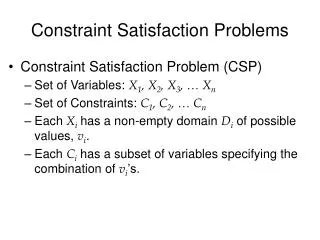
3. Posing a CSP • A set of variables V1, …, Vn • A domain over each variable D1,…,Dn • A set of constraint relations C1,…,Cm between variables which indicate permitted combinations • Goal is to find an assignment to each variable such than none of the constraints are violated

4. A A B B C C D D Constraint Graphs • Nodes = variables • Edges = constraints • Example: map coloring

5. X X Y Z Y Z Hyper graph Primal constraint graph N-ary Constraint Graphs • Example: • Variables: X=[1,2] Y=[3,4] Z=[5,6] • Constraints: X + Y = Z (Roman Barták, 1998 )

6. Making a Binary CSP • Can convert n-ary constraint C into a unary constraint on new variable Vc • Dc = cartesian product of vars in C • Can convert n-ary CSP into a binary CSP • Create var Vc for each constraint C (as above) • Domain Dc = cartesian product – tuples that violate C • Add binary equivalence constraints between new variables Vc, Vc’:C,C’ share var X Vc,Vc’ must agree on X

7. X XYZ Y Z XYZ= [(1,3,5),(1,3,6), (1,4,5),(1,4,6), (2,3,5),(2,3,6) (2,4,5),(2,4,6)] Making a Unary Constraint • Variables: X=[1,2] Y=[3,4] Z=[5,6] • Constraints: X + Y = Z (Roman Barták, 1998 )

8. Making a Unary Constraint • Variables: X=[1,2] Y=[3,4] Z=[5,6] • Constraints: X + Y = Z X XYZ Y Z XYZ= [(1,4,5), (2,3,5), (2,4,6)] (Roman Barták, 1998 )

9. X XYZ Y Y Z WY Dual constraint graph W Making a Binary CSP • Variables: X=[1,2] Y=[3,4] Z=[5,6] W=[1,3] • Constraints: X + Y = Z, W<Y (Roman Barták, 1998 )

10. XYZ Y WY Dual constraint graph Making a Binary CSP • Variables: X=[1,2] Y=[3,4] Z=[5,6] W=[1,3] • Constraints: X + Y = Z, W<Y X Y Z W (Roman Barták, 1998 )

11. Contents • Representations • Solving with Tree Search and Heuristics • Constraint Propagation • Tree Clustering

12. Generate and Test • Generate each possible assignment to the variables and test if constraints are satisfied • Exponential possibilities: O(d n) • Simple but extremely wasteful!

13. DFS and Backtracking • Depth first search • Levels represent variables • Branches off nodes represent a possible instantiations of variables • Test against constraints after every variable instantiation and backtrack if violation • Incrementally attempts to extend partial solution • Whole subtrees eliminated at once

14. Example V1 red green blue V2 V3 red red green (*,*,*)

15. Example V1 red green blue V2 V3 red red green (*,*,*) (r,*,*)

16. Example V1 red green blue V2 V3 red red green (*,*,*) (r,*,*) (r,r,*)

17. Example V1 red green blue V2 V3 red red green (*,*,*) (r,*,*) (g,*,*) (r,r,*) (g,r,*)

18. Example V1 red green blue V2 V3 red red green (*,*,*) (r,*,*) (g,*,*) (r,r,*) (g,r,*) (g,r,r) (g,r,g)

19. Example V1 red green blue V2 V3 red red green (*,*,*) (r,*,*) (g,*,*) (b,*,*) (r,r,*) (g,r,*) (b,r,*) (g,r,r) (g,r,g) (b,r,r) (b,r,g)

20. Forward Checking • Backtracking is still wasteful • A lot of time is spent searching in areas where no solution remains • Ex. setting V4 to value X1 eliminates all possible values for V8 under the given constraints • Can cause thrashing • Forward checking removes restricted values from the domains of all uninstantiated variables • If a domain becomes empty backtracking is done immediately

21. Heuristics • The search can usually be sped up by searching intelligently: • Most-constrained variable: Expand subtree of variables that have the fewest possible values within their domain first • Most-constraining variable: Expand subtree of variables which most restrict others first • Least-constraining value: Choose values that allow the most options for the remaining variables first

22. Contents • Representations • Solving with Tree Search and Heuristics • Constraint Propagation • Tree Clustering

23. Constraint Propagation • A preprocessing step to shrink the CSP • Constraints are used to gradually narrow down the possible values from the domains of the variables • A singleton may result • If the domains of each variable contain a single value we do not need to search

24. Arc Consistency • Arc (Vi,Vj) in a constraint graph is arc consistent if for every value of Vi there is some value that is permitted for Vj • Algorithm: • Complexity O(ed3) do foreach edge (i,j) delete values from Di that cause Arc(Vi,Vj) to fail while deletions

25. Example V1 green V2 V3 red green blue green blue Consider edge (1,3)

26. Example V1 green V2 V3 red green blue green blue Consider edge (3,1)

27. Example V1 green V2 V3 red green blue green blue Consider edge (2,1)

28. Example V1 green V2 V3 red green blue green blue Consider edge (2,3)

29. Example V1 green V2 V3 red green blue green blue Consistent and a singleton!

30. Levels of Consistency • Algorithms we have seen before are combinations of tree search and arc consistency: Generate and Test Backtracking Forward Checking Partial Lookahead Full Lookahead Really Full Lookahead TS BT = TS + AC 1/5 FC = TS + AC 1/4 PL = FC + AC 1/3 FL = FC + AC 1/2 RFL = FC + AC (Nadel, 1988)

31. Backtracking • Given: • check(i,Xi,j,Xj): true if Vi = Xi and Vj = Xj is permitted by constraints • revise(i,j): true if Di is empty after making Arc(Vi,Vj) = true function BT(i,var) for(var[i]=Di) CONSISTENT = true for(j=1:i-1) CONISITENT = check(i,var[i],j,var[j]) end if CONSISTENT if i==n disp(var) else BT(i+1,var) end function BT(i) EMPTY_DOMAIN = check_backward(i) if ~EMPTY_DOMAIN for(var[i]=Di) Di = var[i] if i==n disp(var) else BT(i+1) end function check_backward(i) for(j=1:i-1) if revise(i,j) return true end return false

32. Forward Checking function FC(i) EMPTY_DOMAIN = check_forward(i) if ~EMPTY_DOMAIN for(var[i]=Di) Di = var[i] if i==n disp(var) else FC(i+1) end function check_forward(i) if i>1 for(j=i:n) if revise(j,i-1) return true end return false • Similar to backtracking except more arc-consistency

33. Levels of Consistency Generate and Test Backtracking Forward Checking Partial Lookahead Full Lookahead Really Full Lookahead TS BT = TS + AC 1/5 FC = TS + AC 1/4 PL = FC + AC 1/3 FL = FC + AC 1/2 RFL = FC + AC (Nadel, 1988)

34. A Stronger Degree of Consistency • A graph is K-consistent if we can choose values for any K-1 variables that satisfy all the constraints, then for any Kth variable be able to assign it a value that satisfies the constraints • A graph is strongly K-consistent if J-consistent for all J < K • Node consistency is equivalent to strong 1-consistency • Arc consistency is equivalent to strong 2-consistency

35. Towards Backtrack Free Search • A graph that has strong n-consistency requires no search • Acquiring strong n-consistency is exponential in the number of variables (Cooper, 1989) • For a general graph that is strongly k-consistent (where k < n) backtracking cannot be avoided

36. (*,*,*) (r,*,*) (r,r,*) … Example V1 red green V2 V3 red green green blue Arc consistent, yet a search will backtrack!

37. Constraint Graph Width V1 V1 V2 V2 V3 V3 V1 V2 V3 V1 V3 V1 V2 • The nodes of a constraint graph can be ordered V2 V3 V3 V2 V3 V1 V2 V1 1 1 1 2 1 2  1 • The width of a node in an ordered graph is equal to the number of incoming arcs from higher up nodes • The width of an ordered graph is the max width of its vertices • The width of a constraint graph is the min width of each of its orderings

38. Backtrack Free Search • Theorem: If a constraint graph is strongly K-consistent, and K is greater than its width, then there exists a search order that is backtrack free • K>2 consistency algorithms add arcs requiring even greater consistency • If a graph has width 1 we can use node and arc consistency to get strong 2-consistency without adding arcs • All tree structured constraint graphs have width 1 (Freuder 1988)

39. Contents • Representations • Solving with Tree Search and Heuristics • Constraint Propagation • Tree Clustering

40. Tree Clustering Motivation • Tree structured constraint graphs can be solved without backtracking • We would like to turn non-tree graphs into trees by grouping variables • The grouped variables themselves become smaller CSP’s • Solving a CSP is exponential in the worst case so reducing the number of variables we consider at once is also important • If we want the CSP for many queries it is worth investing more time in restructuring it (Dechter, 1988)

41. ABC AEF AC AE ACE CDE CE Join graph/tree Redundancy • Constraints in the dual graph are equalities • Variables: A, B, C, D, E, F • Constraints: (ABC), (AEF), (CDE), (ACE) A ABC AEF C E AC AE ACE CDE CE

42. Tree Clustering • If the dual graph cannot be reduced to a join tree we can still make it acyclic: • Condition for acyclicity: A CSP is acyclic iff its primal graph is chordal and conformal • Given a primal graph its dual can be made acyclic: • Triangulate graph to make it chordal • The maximal cliques are constraints/nodes in the new dual graph (Beeri, 1983)

43. Triangulation • Use maximum cardinality search (m-ordering) to order the nodes • Add an edge between any two nonadjacent nodes that are connected by nodes higher in the ordering (Tarjan, 1984)

44. The Algorithm • Build the primal graph for the CSP • O(n2) • Triangulate • O(n2) • Use maximal cliques as new nodes in dual graph • O(n) • Remove any redundancies in the new graph • O(n)

45. BD BD D D D D D AD DE AD DE A A E E C C AC CE AC CE Example • Variables: A, B, C, D, E • Constraints: (A,C), (A,D), (B,D), (C,E), (D,E) Still cyclic!

46. B E A E C D C D C A B A B D E Order: E, D, C, A, B Example • Variables: A, B, C, D, E • Constraints: (A,C), (A,D), (B,D), (C,E), (D,E)

47. E BD BD D D D C D ACD CDE ACD CDE A B CD CD Example • Variables: A, B, C, D, E • Constraints: (A,C), (A,D), (B,D), (C,E), (D,E) Acyclic!

48. Solving the CSP • Solve each node of the tree as a separate small CSP • This can be done in parallel • The solutions to each node constitute the domain of that node in the tree • O(d m) • Use arc consistency to reduce the domains of each node • Solve the entire CSP without backtracking

49. Appendix

50. Example CSP’s • N-queens • Map coloring • Cryptoarithmatic • Wireless network base station placement • Object recognition from image features