Understanding Constraint Satisfaction Problems (CSPs) and Their Applications in AI
This chapter provides an in-depth look into Constraint Satisfaction Problems (CSPs), where the state is defined by variables with specific values from domains. CSPs involve goal tests based on constraints determining allowable variable combinations. Examples include map-coloring tasks and cryptarithmetic puzzles, showcasing methods like backtracking and heuristics (MRV, degree, and LCV) to enhance search efficiency. Key characteristics and varieties of CSPs are discussed, including discrete and continuous variables, binary and higher-order constraints. The significance of effective algorithms for solving CSPs in artificial intelligence is emphasized.

Understanding Constraint Satisfaction Problems (CSPs) and Their Applications in AI
E N D
Presentation Transcript
Constraint Satisfaction Problems Chapter 5 Section 1 – 3
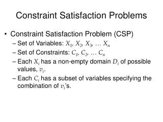
Constraint satisfaction problems (CSPs) • CSP: • state is defined by variablesXi with values from domainDi • goal test is a set of constraints specifying allowable combinations of values for subsets of variables • Allows useful general-purpose algorithms with more power than standard search algorithms
Example: Map-Coloring • VariablesWA, NT, Q, NSW, V, SA, T • DomainsDi = {red,green,blue} • Constraints: adjacent regions must have different colors • e.g., WA ≠ NT
Example: Map-Coloring • Solutions are complete and consistent assignments, e.g., WA = red, NT = green,Q = red,NSW = green,V = red,SA = blue,T = green
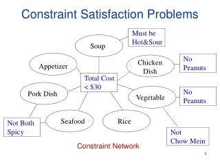
Constraint graph • Binary CSP: each constraint relates two variables • Constraint graph: nodes are variables, arcs are constraints
Varieties of CSPs • Discrete variables • finite domains: • n variables, domain size d O(d n) complete assignments • e.g., 3-SAT (NP-complete) • infinite domains: • integers, strings, etc. • e.g., job scheduling, variables are start/end days for each job: StartJob1 + 5 ≤ StartJob3 • Continuous variables • linear constraints solvable in polynomial time by linear programming
Varieties of constraints • Unary constraints involve a single variable, • e.g., SA ≠ green • Binary constraints involve pairs of variables, • e.g., SA ≠ WA • Higher-order constraints involve 3 or more variables, • e.g., SA ≠ WA ≠ NT
Example: Cryptarithmetic • Variables: F T U W R O X1 X2 X3 • Domains: {0,1,2,3,4,5,6,7,8,9} {0,1} • Constraints: Alldiff (F,T,U,W,R,O) • O + O = R + 10 ·X1 • X1 + W + W = U + 10 · X2 • X2 + T + T = O + 10 · X3 • X3 = F, T ≠ 0, F≠ 0
NxD WA WA WA NT T [NxD]x[(N-1)xD] WA NT WA NT WA NT NT WA Standard search formulation • Let’s try the standard search formulation. • We need: • Initial state: none of the variables has a value (color) • Successor state: one of the variables without a value will get some value. • Goal: all variables have a value and none of the constraints is violated. N layers Equal! N! x D^N There are N! x D^N nodes in the tree but only D^N distinct states??
NT WA WA NT = Backtracking (Depth-First) search • Special property of CSPs: They are commutative: • This means: the order in which we assign variables • does not matter. • Better search tree: First order variables, then assign them values one-by-one. D WA WA WA WA NT D^2 WA NT WA NT D^N
Improving backtracking efficiency • General-purpose methods can give huge gains in speed: • Which variable should be assigned next? • In what order should its values be tried? • Can we detect inevitable failure early? • We’ll discuss heuristics for all these questions in the following.
Which variable should be assigned next?minimum remaining values heuristic • Most constrained variable: choose the variable with the fewest legal values • a.k.a. minimum remaining values (MRV) heuristic • Picks a variable which will cause failure as soon as possible, allowing the tree to be pruned.
Which variable should be assigned next? degree heuristic • Tie-breaker among most constrained variables • Most constraining variable: • choose the variable with the most constraints on remaining variables (most edges in graph)
In what order should its values be tried? least constraining value heuristic • Given a variable, choose the least constraining value: • the one that rules out the fewest values in the remaining variables • Leaves maximal flexibility for a solution. • Combining these heuristics makes 1000 queens feasible
Rationale for MRV, DH, LCV • In all cases we want to enter the most promising branch, but we also want to detect inevitable failure as soon as possible. • MRV+DH: the variable that is most likely to cause failure in a branch is assigned first. The variable must be assigned at some point, so if it is doomed to fail, we’d better found out soon. E.g X1-X2-X3, values 0,1, neighbors cannot be the same. • LCV: tries to avoid failure by assigning values that leave maximal flexibility for the remaining variables. We want our search to succeed as soon as possible, so given some ordering, we want to find the successful branch.
Can we detect inevitable failure early? forward checking • Idea: • Keep track of remaining legal values for unassigned variables that are connected to current variable. • Terminate search when any variable has no legal values
Forward checking • Idea: • Keep track of remaining legal values for unassigned variables • Terminate search when any variable has no legal values
Forward checking • Idea: • Keep track of remaining legal values for unassigned variables • Terminate search when any variable has no legal values
Forward checking • Idea: • Keep track of remaining legal values for unassigned variables • Terminate search when any variable has no legal values
b e a c d 2) Consider the constraint graph on the right. The domain for every variable is [1,2,3,4]. There are 2 unary constraints: - variable “a” cannot take values 3 and 4. - variable “b” cannot take value 4. There are 8 binary constraints stating that variables connected by an edge cannot have the same value. a) [5pts] Find a solution for this CSP by using the following heuristics: minimum value heuristic, degree heuristic, forward checking. Explain each step of your answer. CONSTRAINT GRAPH
b e a c d 2) Consider the constraint graph on the right. The domain for every variable is [1,2,3,4]. There are 2 unary constraints: - variable “a” cannot take values 3 and 4. - variable “b” cannot take value 4. There are 8 binary constraints stating that variables connected by an edge cannot have the same value. a) [5pts] Find a solution for this CSP by using the following heuristics: minimum value heuristic, degree heuristic, forward checking. Explain each step of your answer. MVH a=1 (for example) FC+MVH b=2 FC+MVH c=3 FC+MVH d=4 FC e=1 CONSTRAINT GRAPH
Constraint propagation • Forward checking only checks consistency between assigned and non-assigned states. How about constraints between two unassigned states? • NT and SA cannot both be blue! • Constraint propagation repeatedly enforces constraints locally
Arc consistency • Simplest form of propagation makes each arc consistent • X Y is consistent iff for every value x of X there is some allowed y of Y consistent arc. constraint propagation propagates arc consistency on the graph.
Arc consistency • Simplest form of propagation makes each arc consistent • X Y is consistent iff for every value x of X there is some allowed y inconsistent arc. remove blue from source consistent arc.
Arc consistency • Simplest form of propagation makes each arc consistent • X Y is consistent iff for every value x of X there is some allowed y • If X loses a value, neighbors of X need to be rechecked: i.e. incoming arcs can become inconsistent again (outgoing arcs will stay consistent). this arc just became inconsistent
Arc consistency • Simplest form of propagation makes each arc consistent • X Y is consistent iff for every value x of X there is some allowed y • If X loses a value, neighbors of X need to be rechecked • Arc consistency detects failure earlier than forward checking • Can be run as a preprocessor or after each assignment # arcs • Time complexity: O(n2d3) d^2 for checking, each node can be checked d times at most
Arc Consistency • This is a propagation algorithm. It’s like sending messages to neighbors on the graph! How do we schedule these messages? • Every time a domain changes, all incoming messages need to be re-send. Repeat until convergence no message will change any domains. • Since we only remove values from domains when they can never be part of a solution, an empty domain means no solution possible at all back out of that branch. • Forward checking is simply sending messages into a variable that just got its value assigned. First step of arc-consistency.
Constraint Propagation Algorithm • Maintain all allowed values for each variable. • At each iteration pick the variable with the fewest remaining values • For variables with equal nr of remaining values, break ties by checking • which variable has the largest nr of constraints with unassigned variables • After we picked a variables, tentatively assign it to each of the remaining • values in turn and run constraint propagation to convergence. • (This involves iteratively making all arcs consistent that flow into domains that • just have been changed, beginning with the neighbors of • the variable you just assigned a value to and iterating until no more changes occur.) • Among all checked values, pick the one that removed the least values • from other domains using constraint propagation. • Now run constraint propagation once more (or recall it from memory) for the • assigned value and remove the the values from the domains of the other variables. • When domains get empty, back out of that branch. • Iterate until a solution has been found. • (as an alternative you only do constraint propagation after an assignment to prune • domains of other variables but avoid doing it for all values. Use simply forward • checking with the LCV heuristic to pick a value)
Try it yourself [R,B,G] [R,B,G] [R] [R,B,G] [R,B,G] Use all heuristics including arc-propagation to solve this problem.
B G R R G B a priori constrained nodes B R G B G B R G G R B Note: After the backward pass, there is guaranteed to be a legal choice for a child node for any of its leftover values. This removes any inconsistent values from Parent(Xj), it applies arc-consistency moving backwards.
Local search for CSPs • Note: The path to the solution is unimportant, so we can apply local search! • To apply to CSPs: • allow states with unsatisfied constraints • operators reassign variable values • Variable selection: randomly select any conflicted variable • Value selection by min-conflicts heuristic: • choose value that violates the fewest constraints • i.e., hill-climb with h(n) = total number of violated constraints
Example: 4-Queens • States: 4 queens in 4 columns (44 = 256 states) • Actions: move queen in column • Goal test: no attacks • Evaluation: h(n) = number of attacks
Hard satisfiability problems • A,B,C,D,E can take value (true, false). • A=true means that A must be false. • (B A C) =true means that B=true or A=false or C=false • Consider random conjunctions of constraints: (D B C)=true (B A C)=true (C B E)=true (E D B)=true (B E C)=true • We want to find assignments that make all constraints true m = number of clauses (5) n = number of symbols (5) • Hard problems seem to cluster near m/n = 4.3 (critical point) Implementing algorithms for random 3-SAT problems will be your project
Hard satisfiability problems • Median runtime for 100 satisfiable random 3-CNF sentences, n = 50