Branch-and-Bound
Branch-and-Bound. In this handout, Summary of branch-and-bound for integer programs Updating the lower and upper bounds for OPT(IP) Summary of fathoming criteria Which variable to branch on? Which open subproblem to solve first? Optimality test Branch-and-bound applied to


Branch-and-Bound
E N D
Presentation Transcript
Branch-and-Bound In this handout, • Summary of branch-and-bound for integer programs • Updating the lower and upper bounds for OPT(IP) • Summary of fathoming criteria • Which variable to branch on? • Which open subproblem to solve first? • Optimality test • Branch-and-bound applied to • binary integer programs • mixed integer programs
Examples of the main steps of the algorithm will be given based on the following solution tree S7 Z=52 intF3 S3 Z=60.5 S1 Z=68.7 S8 Z=54.4 F1 S4 Infeas. F2 S9 Z=66.7 All Z=75.4 S5 Z=68.3 S10 Z=59 intF3 S2 Z=70.1 S11 Z=62.9 S6 Z=64.5
Updating the lower and upper bounds for OPT(IP) • The best integer solution found so far is stored as incumbent. The optimal value of the incumbent is denoted by Z*. Z* is the tightest lower bound we have for OPT(IP) in the current iteration: OPT(IP) ≥ Z* . In our example, Z* = 59 (optimal value of S10). • Consider all those subproblems such that (i) the subproblem is unfathomed; (ii) at least one of its child-subproblems is not solved yet. In our example, those subproblems are S6, S9, S11. Let Z’ be the largest LP optimal value for this kind of subproblems. Then Z’ is the tightest upper bound for OPT(IP) in the current iteration: OPT(IP) Z’ . In our example, Z’ = 66.7 (LP optimal value of S9).
Summary of fathoming criteria Fathom a subproblem if at least one of the following is true: • Criterion F1: The LP optimal value of the subproblem is Z*, where Z* is the optimal value of the current incumbent. In our example, S8 is fathomed based on F1 (54.4 < Z*=59). • Criterion F2: The subproblem is infeasible. In our example, S4 is fathomed based on F2. • Criterion F3: The optimal solution of the subproblem is integral. In our example, S7 and S10 are fathomed based on F3.
Which open (unfathomed) subproblem to solve first? Possible natural choices: • Option 1: The subproblem with the best LP value. This subproblem is the most promising one • to create an incumbent with higher Z* value; • to contain an optimal IP solution. • Option 2:The most recently created subproblem. We don’t need to start the simplex method from scratch to solve this subproblem; it is solved by reoptimizing the solution of its parent-subproblem. The second option is normally the preferred choice because it makes the algorithm more time-efficient.
Summary of branch-and-bound Steps for each iteration: • Branching: Among the unfathomed subproblems, select the one that was created most recently. (Break ties according to which has larger LP value.) Choose a variable xi which has a noninteger value xi* in the LP solution of the subproblem. Create two new subproblems by adding the respective constraints xi xi* and xi ≥ xi* . • Bounding: Solve the new subproblems, record their LP solutions. Based on the LP values, update the incumbent, and the lower and upper bounds for OPT(IP) if necessary. • Fathoming: For each new subproblem, apply the three fathoming tests. Discard the subproblems that are fathomed. • Optimality test:If there are no unfathomed subproblems left then return the current incumbent as optimal solution (if there is no incumbent then IP is infeasible.) Otherwise, perform another iteration.
Finding a first incumbent quickly • Recall that having an incumbent allows us to fathom subproblems (Criterion F1). • But it might take many iterations until branch-and-bound finds a first incumbent (a subproblem which has an integer LP solution). • To accelerate the process, a first incumbent is often found by applying a fast heuristic algorithm to the problem. • For example, to solve the Traveling Salesman Problem by Branch-and-Bound, we can start by applying the Nearest Neighbor algorithm to find a first incumbent.
How the upper bound on OPT(IP) can be used • In practice, branch-and-bound is pretty fast most of the time. • But sometimes it might get really slow. (In the worst-case scenario it is still exponential-time.) • What can we do if the branch-and-bound couldn’t find an optimal solution after struggling several hours on the problem? • Recall the tightest lower and upper bounds on OPT(IP) in the current iteration: Z* OPT(IP) Z’ . • What can we say about the current incumbent based on these bounds?Let k = Z’ / Z*. Then That is, the current incumbent is at most k times worse than the optimal solution. If k is close to 1, then the current incumbent will be a pretty good solution. E.g., if Z*=100, Z’=102, then the current incumbent is at most 1.02 times worse than the optimal solution.
Branch-and-bound applied to binary integer programs The only modification: When branching on a binary variable xi, which has a fractional value xi* in the current LP solution, the two new subproblems are created by setting xi = 0 and xi = 1 . Branch-and-bound applied to mixed integer programs The only modification: Branch only on integer-restricted variables.