Download
1 / 30
300 likes | 381 Vues
Explore the synthesis of empirical evidence on ETS and lung cancer risk through adjusted likelihoods, hierarchical models, and systematic adjustments. Understand parametric adjustments, classification probabilities, data gathering, and misclassifications.

E N D
Adjusted Likelihoods for Synthesizing Empirical Evidence from Studies that Differ in Quality and Design: Effects of Environmental Tobacco Smoke Kerrie Mengersen, Newcastle Aust Robert Wolpert, Duke USA
Is ETS associated with lung cancer? 1981: First studies published (Hirayama, Garfinkel)1986: First meta-analyses (Wald, NRC)1992: EPA Review of 29 studies NHMRC Review (Australia)1994: OSHA Review2002: Boffetta review of 51 studies
Individual studies Exposed Unexposed Case Control N
A common measure: log odds ratio Cohort Studies Variety of ways to extract information about e amid nuisance parameters. Bayesian approach? Eg, Jeffrey’s prior Be(1/2,1/2) on pc|e,pc|e Then eLOR ~ N(m,s2)
A common measure: log odds ratio Case Control Studies • Only have indirect evidence about pc|e, pc|e • If we know pc and pe in target population, then • pc|e=pe|c pc / pe and similarly for pc|e • Also if the outcome is ‘rare’, the relative risk and the odds ratio are approximately equal, so which does not depend on collateral quantities
Exchangeable combination of evidence • Simple pooling: same cond’l exposure probs Cohort studies Case control studieseLOR = 0.70 ± 0.12 eLOR = 0.17 ± 0.05 • Fixed effects: same ei=e for each study iIeLOR = 0.21 ± 0.05 (RR=1.23) • Random effects: same overall eeLOR = 0.28 ± 0.20 (RR=1.32) • Boffetta (2002): Overall RR 1.25 (1.15-1.37)
Exchangeable hierarchical models • Model variation in study-specific parameters pi explicitly • Exchangeable implies cond’ly independent random vectors given the hyperparameter q • Write e as a function of q • Then the joint posterior for e, q and all pi can be factored as p(de) p(dq|e) • The marginal likelihood is thusLEHM = [ Pi Li(pi) p(dpi|q) ] p(dq|e)
Exchangeable hierarchical model likelihood Reduces to • RE for q=(m,t,s) and normal logistic conditional distributions p(dpi|q) • FE for q=e and beta conditional distributions p(dpic|e|q),p(dpie|c|q) • Simple pooling for q=(pce,pce,pce,pce) with unit point masses p(dpi|q) at pi=q.
Partially exchangeable hierarchical model Studies are exchangeable within known groups but the G groups may differ systematically among themselves e ~ p(de); q ~ p(dq|e);qg ~ p(dqg|q); qi~p(dqi|qg) Normal priors: e~N(0,t2), eg~N(e,sg2), ei~N(eg,si2)
1992 EPA results Country Gp All Studies Tiers 1-2Greece 2.01 (1.42,2.84) 1.92 (1.13,3.23)Hong Kong 1.48 (1.21,1.81) 1.61 (1.25,2.07)Japan 1.41 (1.18,1.69) 1.39 (1.16,1.66)USA 1.19 (1.04,1.35) 1.23 (1.04,1.42)W. Europe 1.17 (0.84,1.62) 1.17 (0.85,1.64)China 0.95 (0.81,1.12)
Synthesizing heterogeneous evidence • Threshold exclusion • Weighted likelihood functions • Block mixtures • Mixtures • Hierarchical models • Systematic adjustment of likelihoods
Adjusting the likelihood • Parametric adjustment:LiAdj(q) = Li(f(q,ai)eg, Shift in binomial probability parameter q by setting f(q,ai)=q+ai • Uncertain adjustment:ai is uncertain so has (informative) prior pia(dai|q), soLiAdj(q) = Li(f(q,ai) pia(dai|q)
Adjustment in the ETS studies • True fraction pijkl of ith population with case status i, exposure status j, elibility status k [eg, pices is true fraction of cases, exposed, smokers] • True classification probabilitiesqi=(qice,qice,qice,qice) • Apparent classification probabilities(qice,qice,qice,qice)
Eligibility violation Change of notation: c,C; e,E; s,S Suppress superscript i for each study qceS = aS|ces pces + aceS|ceS pceS + ae|cES pcES + ac|CeS pCeS (Similarly for qcES, qCeS ,qCES ) So we want (pces, pcEs, pCes, pCEs)
Gathering the evidence • EPA Review gives us ps for each study • Get pe|s from pe|S and K=pespES / peSpEs (3, Lee) • Take pc|es = pc|Es = Rspc|S(Rs is RR lung cancer among active smokers)Write pc=pc|s ps + pc|s pS = pc|S(psRs+pS)Thus pc|s = pcRs/psRs+1-ps)and pc|s = pc/(psRs+1-ps ) • This gives us (pis,pie|s,pic|es,pic|Es) so we can find all four required probabilities for each study
Still on eligibility violation: gathering the evidence • We still need p`S’|sLee, EPA: ~ 5% of eversmokers deny smoking.Mixed evidence of dependene on case status; we ignore this.Little evidence of dependence on exposure status; we ignore this. • EPA assigns ‘penalty points’ Ai ranging from –0.5 (bonus) to +1.0 for each study’s control of this bias. • So we takeaiS|ces= aiS|cEs = aiS|Ces = aiS|CEs = 0.05 2Ai
Misclassification of exposure • We want p`e’|E and p`E’|e • Some studies report the other probs eg pE|`e’so use Bayes theorem to invert • Friedman’83: 47% of currently nonsmoking wives have <1 hr/day exposure at home. 40-50% women with nonsmoking spouses have significant ETS exposure outside the home.Lee’92: ‘not a major issue’Jarvis et al’01: good surrogate • We take pE|`e’ = 0.25, pe|`e’=0.10
Misclassification of lung cancer • We need p`c’|c, p`C’|c • No evidence that these differ w.r.t. ETS exposure among nonsmokers • Lee: 30-40% lung cancers seen at autopsy are missed clinically • Thus we take p`c’|c=0.35. • EPA: ‘penalty points’ Bi from –0.5 to +2.5 for each study’s control of this bias. • So we take aiE|ceS = aiE|CeS = .19 2Bi -2.5aie|CES = aie|CES = .14 2Bi-2.5
Misclassification of exposure (cont.) • Lee: 22.5% report exposure: p`e’ = 0.225EPA: rates from 15% to 87% in studies • We take p`e’ = 0.36 • Thus we calculate p`E’|e = 0.19, p`e’|E=0.14 • Reduce by fraction Ci of histologically verified cases, given by the EPA • So we take aic|CeS = aic|CES = 0 aiC|ceS = aiC|cES = .35 (1-Ci)
ei Study-specific LOR Adjusted conditional ‘true’ probabilities pc|e, pc|E, pC|e, pC|E a qce, qcE, qCe, qCE Apparent classificationprobabilities nce , ncE, nCe, nCE Observed data
Hierarchical prior distribution qi can be recovered from qic=qice+qicE, qie=qice+qiCe and eiLOR so we construct a joint distribution for q from that of qc, qe, e. • log(qc/qe) ~ N(mg, 0.5) log(mg) ~ N(m 25/105, 0.5)low precision, little prior opinion on nonsmokers’ cancer rates • log(qie/qiE)~N(me=log(.36/.64)=-0.57,0.842) p`e’ 0.36; reported apparent exposure rates 15%-87%; calculate variance so that P(0.1<qie<0.75) 0.90
A tale of two studies Tier 4 case control study (Chan, Hong Kong)- evidence about qe but not qc Tier 2 cohort study (Hirayama, Japan)- evidence about qc but not qe
Conclusions • Flexible meta-analysis method that directly adjusts the likelihoods • Requires specific, explicit account of factors for which adjustment is made • Allows quantification and introspection about the impact of quality issues • Allows detailed interpretation