CHAPTER 6 S TOCHASTIC A PPROXIMATION AND THE F INITE- D IFFERENCE M ETHOD

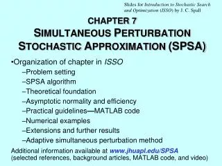
1. Slides for Introduction to Stochastic Search and Optimization (ISSO)by J. C. Spall CHAPTER 6STOCHASTIC APPROXIMATION AND THE FINITE-DIFFERENCE METHOD Organization of chapter in ISSO Contrast of gradient-based and gradient-free algorithms Motivating examples Finite-difference algorithm Convergence theory Asymptotic normality Selection of gain sequences Numerical examples Extensions and segue to SPSA in Chapter 7

2. Motivation for AlgorithmsNot Requiring Gradient of Loss Function • Primary interest here is in optimization problems for which we cannot obtain direct measurements of L/q • cannotuse techniques such as Robbins-Monro SA, steepest descent, etc. • can (in principle) use techniques such as Kiefer and Wolfowitz SA (Chapter 6), genetic algorithms (Chapters 9–10),… • Many such “gradient-free” problems arise in practice • Generic difficult parameter estimation • Model-free feedback control • Simulation-based optimization • Experimental design: sensor configuration

3. Model-Free Control Setup (Example 6.2 in ISSO)

4. Finite Difference SA (FDSA) Method • FDSA has standard “first-order” form of root-finding (Robbins-Monro) SA • Finite difference approximation replaces direct gradient measurement (Chap. 5) • Resulting algorithm sometimes called Kiefer-Wolfowitz SA • Let denote FD estimate of g() at kth iteration (next slide) • Let denote estimate for  at kth iteration • FDSA algorithm has form where ak is nonnegative gain value • Under conditions,  in stochastic sense (a.s.)

5. Finite Difference Gradient Approximation • Classical method for approximating gradients in Kiefer-Wolfowitz SA is by finite differences • FD gradient approximation used in SA recursion as gradient measurement (previous slide) • Standard two-sided gradient approximation at iteration k is where j is p-dimensional with 1 in jth entry, 0 elsewhere • Each computation of FD approximation takes 2p measurements y(•)

6. Shaded Triangle ShowsValid Coefficient Values  and  in Gain Sequences ak = a/(k+1+A) and ck = c/(k+1) (Sect. 6.5 of ISSO) Solid line indicates non-strict border ( or ) and dashed line indicates strict border (>)

7. Example: Wastewater Treatment Problem (Example 6.5 in ISSO) • Small-scale problem with p = 2 • Aim is to optimize water cleanliness and methane gas byproduct • Evaluated algorithms with 50 realizations of N = 2000 measurements • Used FDSA with gains ak = a/(1 + k) and ck = 1/(1 + k)1/6 • Asymptotically optimal decay rates found “best” • Gain tuning chooses a; naïve gain sets a = 1 • Also compared with random search algorithm B from Chapter 2 • Algorithms use noisy loss measurements (same level as in Example 2.7 in ISSO)

8. Mean values ofL() with 95% Confidence Intervals

9. Example: Skewed-Quartic Loss Function(Examples 6.6 and 6.7 in ISSO) • Larger-scale problem with p = 10: ()iis the ith component of B, and pB is an upper triangular matrix of ones • Used N = 1000 measurements; 50 replications • Used FDSA with gains ak = a/(1+k+A) and ck = c/(1+k) • “Semi-automatic” and manual gain tuning • Also compared with random search algorithm B

10. Algorithm Comparison with Skewed-Quartic Loss Function (p = 10) (Example 6.6 in ISSO)

11. Example with Skewed-Quartic Loss: Mean Terminal Values and 95% Confidence Intervals for