Download
1 / 17
170 likes | 302 Vues
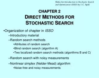
Slides for Introduction to Stochastic Search and Optimization ( ISSO ) by J. C. Spall. CHAPTER 2 D IRECT M ETHODS FOR S TOCHASTIC S EARCH. Organization of chapter in ISSO Introductory material Random search methods Attributes of random search Blind random search (algorithm A)

E N D
Slides for Introduction to Stochastic Search and Optimization (ISSO)by J. C. Spall CHAPTER 2DIRECT METHODS FOR STOCHASTIC SEARCH Organization of chapter in ISSO Introductory material Random search methods Attributes of random search Blind random search (algorithm A) Two localized random search methods (algorithms B and C) Random search with noisy measurements Nonlinear simplex (Nelder-Mead) algorithm Noise-free and noisy measurements
Some Attributes of Direct Random Search with Noise-Free Loss Measurements • Ease of programming • Use of only L values (vs. gradient values) • Avoid “artful contrivance” of more complex methods • Reasonable computational efficiency • Generality • Algorithms apply to virtually any function • Theoretical foundation • Performance guarantees, sometimes in finite samples • Global convergence in some cases
Algorithm A: Simple Random (“Blind”) Search Step 0 (initialization) Choose an initial value of =inside of . Set k = 0. Step 1 (candidate value) Generate a new independent value new(k+1) , according to the chosen probability distribution. If L(new(k+1)) < set = new(k+1). Else take = . Step 2 (return or stop) Stop if maximum number of L evaluations has been reached or user is otherwise satisfied with the current estimate for ; else, return to step 1 with the new k set to the former k+1.
First Several Iterations of Algorithm A on Problem with Solution = [1.0, 1.0]T (Example 2.1 in ISSO)
Functions for Convergence (Parts (a) and(b)) and Nonconvergence (Part (c)) of Blind Random Search (a) Continuous L(); probability density for new is > 0 on = [0, ) (b) Discrete L(); discrete sampling for new with P(new= i) > 0 for i = 0, 1, 2,... (c) Noncontinuous L(); probability density for new is > 0 on = [0, )
Algorithm B: Localized Random Search Step 0 (initialization) Choose an initial value of =inside of . Set k = 0. Step 1 (candidate value) Generate a random dk. Check if . If not, generate new dk or move to nearest valid point. Let new(k+1) be or the modified point. Step 2 (check for improvement) If L(new(k+1)) < set = new(k+1). Else take = . Step 3 (return or stop) Stop if maximum number of L evaluations has been reached or if user satisfied with current estimate; else, return to step 1 with new k set to former k+1.
Algorithm C: Enhanced Localized Random Search • Similar to algorithm B • Exploits knowledge of good/bad directions • If move in one direction produces decrease in loss, add bias to next iteration to continuealgorithm moving in “good” direction • If move in one direction produces increase in loss, add bias to next iteration to move algorithm in opposite way • Slightly more complex implementation than algorithm B
Formal Convergence of Random Search Algorithms • Well-known results on convergence of random search • Applies to convergence of and/or L values • Applies when noise-freeL measurements used in algorithms • Algorithm A (blind random search) converges under very general conditions • Applies to continuous or discrete functions • Conditions for convergence of algorithms B and C somewhat more restrictive, but still quite general • ISSO presents theorem for continuous functions • Other convergence results exist • Convergence rate theory also exists: how fast to converge? • Algorithm A generally slow in high-dimensional problems
Example Comparison of Algorithms A, B, and C • Relatively simple p = 2 problem (Examples 2.3 and 2.4 in ISSO) • Quartic loss function (plot on next slide) • One global solution; several local minima/maxima • Started all algorithms at common initial condition and compared based on common number of loss evaluations • Algorithm A needed no tuning • Algorithms B and C required “trial runs” to tune algorithm coefficients
Multimodal Quartic Loss Function for p = 2 Problem (Example 2.3 in ISSO)
Example 2.3 in ISSO (cont’d): Sample Means of Terminal Values – L()in Multimodal Loss Function(with Approximate 95% Confidence Intervals)
Examples 2.3 and 2.4 in ISSO (cont’d):Typical Adjusted Loss Values ( – L()) and Estimates in Multimodal Loss Function (One Run)
Random Search Algorithms with Noisy Loss Function Measurements • Basic implementation of random search assumes perfect (noise-free) values of L • Some applications require use of noisy measurements: y() = L() + noise • Simplest modification is to form average of y values at each iteration as approximation to L • Alternative modification is to set threshold > 0 for improvement before new value is accepted in algorithm • Thresholding in algorithm B with modified step 2: Step 2 (modified) If y(new(k+1)) < set = new(k+1). Else take = . • Very limited convergence theory with noisy measurements
Nonlinear Simplex (Nelder-Mead) Algorithm • Nonlinear simplex method is popular search method (e.g., fminsearchin MATLAB) • Simplex is convex hull of p + 1 points in p • Convex hull is smallest convex set enclosing the p + 1 points • For p = 2 convex hull is triangle • For p = 3 convex hull is pyramid • Algorithm searches for by moving convex hull within • If algorithm works properly, convex hull shrinks/collapses onto • No injected randomness (contrast with algorithms A, B, and C), but allowance for noisy loss measurements • Frequently effective, but no general convergence theory and many numerical counterexamples to convergence
Steps of Nonlinear Simplex Algorithm Step 0 (Initialization)Generate initial set of p + 1 extreme points in p, i (i = 1, 2, …, p + 1), vertices of initial simplex Step 1 (Reflection)Identify where max, second highest, and min loss values occur; denote them by max, 2max, and min, respectively. Let cent = centroid (mean) of all i except for max. Generate candidate vertex refl by reflecting max through cent using refl = (1 + )cent max ( > 0). Step 2a (Accept reflection) If L(min) L(refl) < L(2max), then refl replaces max; proceed to step 3; else go to step 2b. Step 2b (Expansion) If L(refl) < L(min), then expand reflection using exp = refl + (1 )cent, > 1; else go to step 2c. If L(exp) < L(refl), then expreplaces max; otherwise reject expansion and replace max by refl. Go to step 3.
Steps of Nonlinear Simplex Algorithm (cont’d) Step 2c (Contraction) If L(refl) L(2max), then contract simplex: Either case (i) L(refl) < L(max), or case (ii) L(max) L(refl). Contraction point is cont = max/refl + (1 )cent, 0 1, where max/refl = refl if case (i), otherwise max/refl = max. In case (i), accept contraction if L(cont) L(refl); in case (ii), accept contraction if L(cont) < L(max). If accepted, replace max bycontand go to step 3; otherwise go to step 2d. Step 2d (Shrink) If L(cont) L(max), shrink entire simplex using a factor 0 < < 1, retaining only min. Go to step 3. Step 3 (Termination) Stop if convergence criterion or maximum number of function evaluations is met; else return to step 1.
max max min min cent cent refl 2max 2max refl exp Expansion when L(refl) < L(min) Reflection max max min max min min cont cent cent cent cont cont refl refl refl 2max 2max 2max Shrink after failed contraction when L(refl)< L(max) Contraction when L(refl) L(max) (“inside”) Contraction when L(refl) < L(max) (“outside”) Illustration of Steps of Nonlinear Simplex Algorithm with p = 2