Download
1 / 82
820 likes | 1.01k Vues
Satellite observation systems and reference systems (ae4-e01). Applications E. Schrama. Contents. Preprocessing of observations - example 1: dual frequency ionospheric effect - example 2: tropospheric range delay effect - example 3: normal point compression technique

E N D
Satellite observation systems and reference systems (ae4-e01) Applications E. Schrama
Contents • Preprocessing of observations • - example 1: dual frequency ionospheric effect • - example 2: tropospheric range delay effect • - example 3: normal point compression technique • Global Positioning System • - Precise point positioning services • - Detection of plate tectonics • - Estimation of wet tropospheric delay • International Earth Rotation Service (IERS) • - Earth rotation parameters + LOD • - Interpretation of these Earth rotation variables (AAM) • Satellite altimetry • - Technique, Role of POD, Results • Gravity missions • - GRACE, GOCE and CHAMP
Preprocessing of observations • Oftentimes raw observations are NOT suitable for direct application in parameter estimation algorithms • Raw observations typically contain non Gaussian errors like outliers greater than 3 sigma • Often there are very good reasons to inspect and clean up the data before you put it into an estimation procedure • This topic is much depending on the observation technique, we will just show some well known examples.
Preprocessing example 1 The problem is: how do you eliminate the ionospheric delay from dual frequency range data?
Preprocessing example 2 • The air pressure is 1000 mbar, the air temperature is 20 degrees centigrade, the relative humidity is 50%, what is the dry+wet tropospheric delay of a radio signal as a function of the elevation angle for a station at MSL and 50 degrees latitude. The answer is: • Use the Hopfield model (see Seeber p 45 - 49) to calculate the refractive index • Use the integral over (n-1) ds to compute the path delay • For the latter integral various mapping functions exist
Dry tropospheric delay example This result is entirely depending on the air pressure P, 1% air pressure change (=10 mbar) gives 1% range change. Since air pressure is usually known to within a mbar the dry tropospheric delay error is small. For low elevation angles the delay error increases due to the mapping function uncertainties. Hence elevation cut-off angles are used (typically 10 degrees). m a
Wet tropospheric delay example The wet tropospheric range depends on the relative humidity which varies more rapidly in time and place compared to air pressure. Variations of the order of 50% are possible. As a result the vertical path delay can vary between 5 and 30 cm. The alternative is the use of a multifrequency radiometer system, see Seeber p 49. m a
Normal point compression Case: red crosses is SLR data, there are too many of them and there are clear blunders that we don’t accept in the parameter estimation procedure. Method: Use a compression technique (splines, polynomials, etc) that fit the crosses. Evaluation of the model results in the compression points (the circles). This procedure filters out the noise. Horizontal: time, vertical: range
GPS: precise point positioning • Concept of differencing • Single differencing • Double differencing • Triple differencing • Software • Bernse software • GIPSY JPL • Other software
Concept of differencing • In the GPS system, many observations are made at the “same” time by difference receivers. • All receivers collect pseudo range data, carrier phase data and navigation messages • The Pseudo range navigation allows you to get a approximate solution for receiver coordinates (approx 3 m) • More importantly is that the pseudo range navigation solution allows to synchronize all receiver clocks to the (approx 10 nano seconds, nsec). • The pseudo-range solution requires orbit information • The dual frequency concept results in ionospheric free ranges and carrier phase estimates • From this point on we start to work with “differencing techniques”,
Single differences SAT(1) SAT(2) r1a r2a RCV(a) Single Difference = r1a - r2a
Double differences SAT(1) SAT(2) r2b r1a r2a r1b RCV(b) RCV(a) Double Difference = (r1a - r2a) - (r1b-r2b)
Difference data processing • Single differences (as shown two sheets before this one) are insensitive to receiver clock errors • Double differences are insensitieve to all receiver and satellite clock errors • Triple differences (= differences of double differences at consequetive epochs) reveal jumps in carrier phase data. • Differencing techniques as described above result in observation equations that allow one to solve for coordinate delta’s (improvements) • Available software to do this: GIPSY (JPL) + Bernese SW
GPS to observedeformation around a vulcano on Hawaii Ref: http://www.unavco.org/research_science/science_highlights/kilauea/kilauea.html
Plate Tectonics Source: Unavco Brochure
GPS: Wet troposphere (cm) http://www.gst.ucar.edu/gpsrg/realtime.html
Ionosphere from GPS (TEC) http://www.gst.ucar.edu/gpsrg/realtime.html
Polar motion • Lectures on reference systems explained what it is (Your vocabulary contains : precession, nutation, polar motion) • Typically observed by all space techniques • It is observable because of a differences between reference systems • Satellite and quasars “live” in an inertial system • We stand with both feet on the ground
IERS: Length of day variations The atmosphere (left) and the ocean tides (right) correlate with space geodetic observations of the length of day (LOD) source: NASA
Satellite Altimetry By means of a nadir looking radar we measure the reflection of short pulse in the footprint. This footprint is about 4 to 8 kilometer in diameter. Source: JPL
Pulse reflection power Sent time power Received time
Technical evolution • SKYLAB 1972 NASA 20 m • GEOS-3 1975-1978 NASA 3 m • SEASAT 1978 NASA 2 m • GEOSAT 1985-1990 US Navy 30 cm • ERS-1 1991-1996 ESA 4-10 cm • ERS-2 1995- ESA 4 cm • T/P 1992- NASA/CNES 2 - 3 cm • GFO 2000- US Navy • JASON 2001- NASA/CNES 2 - 3 cm • ENVISAT 2002- ESA
ERS-1 1991-1996 Topex/Poseidon 1992 - ERS-2 1995- Geosat (1985-1990) Recent and operational systems
Doris tracking network Source: CNES
ERS-1/2 tracking + cal/val Source: DEOS
119 121 120 122 T/P sampling