Droplet Dynamics Multi-phase flow modelling
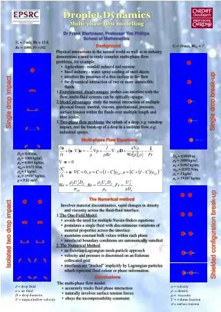
Droplet Dynamics Multi-phase flow modelling. Dr Frank Bierbrauer, Professor Tim Phillips School of Mathematics. U i = 1 m/s , We = 13.8, Re = 1000, Fr =102. Background. U i = 10 m/s, We G = 7. Physical interactions in the natural world as well as in industry

Droplet Dynamics Multi-phase flow modelling
E N D
Presentation Transcript
Droplet Dynamics Multi-phase flow modelling Dr Frank Bierbrauer, Professor Tim Phillips School of Mathematics Ui = 1 m/s, We = 13.8, Re = 1000, Fr =102 Background Ui= 10 m/s, WeG = 7 • Physical interactions in the natural world as well as in industry • demonstrate a need to study complex multi-phase flow • problems, for example: • Agriculture - rainfall induced soil erosion • Steel industry - water spray cooling of steel sheets • involves the presence of a free surface in the flow • the dynamical interaction of two or more immiscible fluids • Experimental disadvantages: probes can interfere with the flow, multi-fluid systems can be optically opaque • Model advantages: study the mutual interaction of multiple physical forces: inertial, viscous, gravitational, pressure, surface tension within the fluids over multiple length and time scales. • Two-phase flow problems: the splash of a drop, e.g. raindrop impact, and the break-up of a drop in a uniform flow, e.g. industrial sprays. Single drop break-up Single drop Impact Multi-phase Flow Equations Dd = 0.001m, rd = 1000 kg/m3, md = 0.001 kg/ms, sad = 0.072 N/m, ra = 1 kg/m3, ma = 1×10⁻⁵ kg/ms, g = 9.81 m/s2 Dd = 0.0049 m, rd = 1000 kg/m3, md = 0.001 kg/ms, sad = 0.072 N/m, ra = 1 kg/m3, ma = 1×10⁻⁵kg/ms The Numerical method • Involves material discontinuities, rapid changes in density and viscosity across the fluid-fluid interface. • The One-Field Model • avoids the need for multiple Navier-Stokes equations • postulates a single fluid with discontinuous variations of material properties across the interface • maintains constant bulk values within each phase • interfacial boundary conditions are automatically satisfied • 2. The Numerical Method • an Eulerian-Lagrangian mesh-particle approach • velocity and pressure is discretised on an Eulerian collocated grid • interfaces are “tracked” implicitly by Lagrangian particles which represent fluid colour or phase information. Isolated two drop impact Shielded configuration break-up Conclusions • The multi-phase flow model: • accurately tracks fluid phase interaction • naturally involves surface tension forces • obeys the incompressibility constraint d = drop fluid a = air fluid D = drop diameter U = impact/inflow velocity u = velocity r = density m = viscosity C = volume fraction s = surface tension