Urban turbulence - flow statistics, dynamics and modelling
520 likes | 729 Vues
Urban turbulence - flow statistics, dynamics and modelling. A numerical study using direct numerical simulations (DNS) over groups of idealized buildings. Omduth Coceal Dept. of Meteorology, Univ. of Reading, UK. Email: o.coceal@reading.ac.uk and Dobre, S.E. Belcher (Reading)

Urban turbulence - flow statistics, dynamics and modelling
E N D
Presentation Transcript
Urban turbulence - flow statistics, dynamics and modelling A numerical study using direct numerical simulations (DNS) over groups of idealized buildings Omduth Coceal Dept. of Meteorology, Univ. of Reading, UK. Email: o.coceal@reading.ac.uk and Dobre, S.E. Belcher (Reading) T.G. Thomas, Z. Xie, I.P. Castro (Southampton) Seminar given at UK Met Office, Exeter, 1 May 2007
Motivation - why DNS? • Field measurements within urban areas are difficult to interpret • Dispersion/ventilation depend on unsteady flow; short timescales • We need a better understanding of turbulence dynamics in urban areas • LES/DNS is a useful tool for obtaining detailed spatial and temporal information • But how can results be useful for simplified modelling?
Outline • Description of numerical simulations • Validation with wind-tunnel data • Flow visualization • Spatial averaging of the data • Statistics for different types of building arrays • Unsteady effects and organized structures • Flow dynamics
Direct numerical simulations • Parallel LES/DNS code developed by T.G. Thomas (Southampton) • Domain size: 16h x 12h x 8h • Resolution: 32 x 32 x 32 gridpoints per cube (also 643 gridpoints per cube on a smaller domain) • Total of 512 x 384 x 256 ~50 million gridpoints • Runs took ~3 weeks on 124 processors on SGI Altix supercomputer
Direct numerical simulations • Boundary conditions • free slip at top of domain • no slip at bottom and on cube surfaces • periodic in horizontal • Reynolds number • 5800 based on Utop and h • Re = 500 • Flow driven by constant body force • Turbulent scales are sufficiently resolved • dissipation captured • good agreement with experiment even without SGS model Coceal et al., BLM (2006) Coceal et al., BLM, to appear Coceal et al., IJC, to appear
Comparisons with experiment Compared with wind-tunnel data from Cheng and Castro (2003) and Castro et al. (2006) stresses spectra velocity pressure
Instantaneous windvectors in y-z plane Mean flow is out of screen 643 gridpoints per cube
Instantaneous windvectors in y-z plane Streamwise circulations visualised in y-z plane (mean flow is out of screen)
Streamwise vorticity in y-z plane Counter-rotating vortex pairs
Mean flow structure Horizontal slices at z = 0.5 h Staggered array Square array Mean flow structure is highly dependent on the building layout
Spatial averaging y h x E.g. Urban canopy models (e.g. Martilli et al. 2002; Coceal & Belcher 2004, 2005) • Don’t resolve horizontal heterogeneity at the building/street scale • Take horizontal averages: resolve vertical flow structure Triple decomposition of velocity field Spatial average of Reynolds-averaged momentum equation - Compute these spatially-averaged quantities from the DNS data
Spatially averaged statistics - uniform arrays Different building layouts, same density (Detailed explanation of this plot in Coceal et al., 2006)
Arrays with random building heights (same density) 0.5hm Compare results with LES performed by Zhengtong Xie (Southampton) Same building density and staggered layout as in uniform array
Spatial averages - mean velocity Velocities are smaller over the random array. The random array exerts more drag. Spatially-averaged velocities are very similar within arrays. Inflection is much weaker in random array.
Spatial averages - stresses In the random array, the peaks are less strong, but still quite pronounced. They occur at the height of the tallest building, not at the mean or modal building height.
Spatial averages - dispersive stresses Profiles of uw component of dispersive stress are very similar below z=h_m.
Spatial fluctuations Qualitatively similar behaviour in the two arrays
Energy partitioning (i) mke dominates above the canopy, but rapidly becomes a negligible fraction of the total k.e. within the canopy, while the fraction of dke and tke both increase. (ii) the fractions of mke, dke and tke for the two arrays are very similar below z=h_m; energy is partitioned roughly in the same proportion. (iii) above the canopy, the tke fraction over the random array is roughly twice as large as that over the regular array.
Buildings of variable heights - TKE TKE from shear layers shed from vertical edges of tallest building dominates above half the mean building height.
Buildings of variable heights - Umag The effect of the tallest building is more pronounced w.r.t. the total velocity magnitude.
Buildings of variable heights - Drag profiles (I) Tallest building (1.72 times the mean building height) exerts 22% of the total drag! The 5 tallest buildings (out of 16) are together responsible for 65% of the drag.
Buildings of variable heights - Drag profiles (II) The shapes of the drag profiles are in general similar for many of the tallest buildings (17.2m, 13.6m, 10.0m) except when they are in the vicinity of a taller building. The profile shapes of the shortest buildings (6.4m and 2.8m) are very different - but these buildings do not exert much drag.
Summary (I): Effect of building geometry on statistics Effects of building layout • Mean flow structure and turbulence statistics vary substantially with layout • Effect of packing density still needs to be properly documented Effects of random building heights: • Less strong shear layer on average • Inflection in spatially-averaged mean wind profile much less pronounced • Larger drag/roughness length • Below the mean building height, spatial averages are very similar to regular array Effects of tall buildings: • Strong shear layers associated with tall buildings - high TKE • They exert a large proportion of the drag • They cause significant wind speed-up lower down the canopy
Quadrant analysis w’ u’ < 0 w’ > 0 u’ > 0 w’ > 0 u’ u’ < 0 w’ < 0 u’ > 0 w’ < 0 Decompose contributions to shear stress <u’w’> according to signs of u’, w’ Ejections (Q2) Sweeps (Q4) Which quadrants contribute most to the Reynolds stress <u’w’> ?
Quadrant analysis Ejections and sweeps dominate They are associated with turbulent organized motions Profiles of fractional frequency and fractional contribution of each quadrant
Quadrant analysis - Exuberance Exuberance From DNS Real field data (Christen, 2005) Exuberance is a measure of how disorganized the turbulence is Magnitude of Exuberance is smallest near canopy top in DNS (uniform building heights) Increases slowly above building canopy, rapidly within canopy
Quadrant analysis - Q2 vs Q4 (I) DNS Indicates character of the organized motions Ejection dominance well above the canopy Sweep dominance close to/within the canopy. Cross-over point is at z = 1.25 h Real field data (Christen, 2005)
Fluctuating velocity vectors in x-z plane Mean flow from left to right. Local mean subtracted from velocity vectors. Ejections and sweeps are associated with eddy structures
Spatial distribution of ejections and sweeps Fluctuating windvectors Red = sweep events Blue = ejection events Unsteady coupling of flow within and above canopy
Two-point correlations Ruu Give information on lengthscale and spatial structure of organized motions Correlation lengthscale increases with height of reference point Small at z = h and within canopy Structures above canopy are inclined; inclination angle is a function of height
Instantaneous structures above buildings in 3d Lower Reynolds number of 1200 (Re = 125, still fully rough flow) Clearly reveals vortex structures (red) and low momentum regions (blue) Vortex cores identified using isosurfaces of negative 2
3d structure of the conditional vortex Hairpin-like conditional vortex obtained by conditional averaging of a large number of instantaneous realisations
Role of canopy-top shear layer y Intermittent impinging of shear layer on downstream buildings drives a recirculation. cf Louka et al. (2000).
Effect of shear layer on flow within canopy Space-time correlation Ruu with negative time delay of -0.4T; ref is at (8, 0.75). T is an eddy turnover time of the largest eddies shed by the cubes.
Shear layers within the canopy z at z = 0.5 h x at y = 0.5 h Interacting vertical shear layers Vortex tilting and stretching
Small-scale circulations within canopy Instantaneous windvectors in y-z plane within a cavity (flow is out of screen )
Summary (II): A conceptual model of the unsteady dynamics Three flow regimes: • Flow well above canopy is a classical rough wall flow and its structure resembles that over a smooth wall boundary layer, although there are quantitative differences. • Flow near the canopy top is dominated by shear layer shed off top of cubes and by larger boundary layer eddies. • Flow within canopy is complicated by interaction of above with shear layers shed off vertical faces of the buildings, vortex stretching and tilting and distortion by roughness.
Vortex identification methods (Jeong & Hussain, JFM 1995 ) Failures of intuitive criteria: • Closed or spiral streamlines • not Galilean invariant • Vorticity magnitude • fails in a shear flow if background shear is appreciable; necessary but not sufficient condition • Local pressure minimum • could also exist in an unsteady irrotational flow without a vortex • vortex could exist without a pressure minimum, due to viscous term • hence, pressure minimum is neither a necessary nor a sufficient condition for existence of a vortex
Vortex identification methods Positive second invariant of the velocity gradient tensor u (Hunt et al. 1988 ) where S and are the symmetric and antisymmetric components of u Hence, Q represents balance between shear strain rate and vorticity magnitude Additionally, the pressure must be lower than its ambient value
The 2vortex identification method (Jeong & Hussain, JFM 1995 ) Take gradient of the Navier-Stokes equation: This equation may be decomposed into symmetric and antisymmetric parts to give: Second equation is vorticity equation
The 2vortex identification method unsteady irrotational straining viscous effects Both ‘mask’ local pressure minimum, hence ignore their contributions (Jeong & Hussain, JFM 1995 ) First equation may be rewritten as: Local pressure minimum in a plane Hessian of pressure has two +ve eigenvalues needs to have two -ve eigenvalues Hence, if eigenvalues are 1, 2, and 3, with 1< 2 < 3, then 2 < 0 within vortex core
Buildings of variable heights - U Wind speed-up around the tall building in relation to the background flow, especially at lower levels.
Time-delayed two-point correlations Ruu with fixed (xref,zref) for successive time delays of 0.1T
Convection velocities cf Castro et al. (2006)
Vortex visualisation by Galilean decomposition Galilean decomposition Vortex structures visualised after subtracting convection velocity (cf Adrian et al. 2000)
POD analysis Vortex reconstructed using first few terms Eigenvalue spectrum Roger Shaw Ned Patton Head-up hairpin-like vortices are energetically dominant