Download
1 / 58
590 likes | 772 Vues
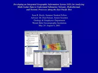
Developing an Integrated Geographic Information System (GIS) for Analyzing Multi-Scalar Data to Understand Submarine Volcanic, Hydrothermal, and Tectonic Processes along the East Pacific Rise. Sean R. Keefe, Summer Student Fellow Advisor: Dr. Dan Fornari, Senior Scientist

E N D
Developing an Integrated Geographic Information System (GIS) for Analyzing Multi-Scalar Data to Understand Submarine Volcanic, Hydrothermal, and Tectonic Processes along the East Pacific Rise Sean R. Keefe, Summer Student Fellow Advisor: Dr. Dan Fornari, Senior Scientist Geology & Geophysics Department Woods Hole Oceanographic Institution May 24 -August 8, 2003
Study Area World Map Showing Northern EPR Inset: Bathymetry of the EPR. (Star locates area of interest.)
Objectives The goal of this summer fellowship research project was to help WHOI geologists visualize, analyze, and interpret the seafloor geology along the EPR by creating a GIS with integrated bathymetric data, navigation data, rock sample data, and digital imagery from recent ship and instrument surveys.
Methods Survey of recent scientific interpretations of the geologic processes occurring at the EPR.
Methods The main steps for creating the new EPR GIS were: 1) Process the raw bathymetric and sidescan sonar grids 2) Process camera tow tables and rock sample tables 3) Process and integrate the digital images with new, interpolated camera tow tables 4) Create groups of related images which can be displayed like dissolve video from within the GIS
I. Processing Bathymetric & Sidescan Sonar Grids To integrate the grids in one coordinate system in ArcGIS, the GMT grids were preprocessed into a common raster format and coordinate system usable in ArcGIS. GMT was used to change the spacing between grid points in decimal degrees, using the following UNIX command: grdedit –A filename.grd The grid file was then converted to an ASCII table, creating a one-column table with rows going from left to right (Figure 4): grd2xyz filename.grd –ZTLA > filename.asc Figure 4. One-column table Figure 5. Header file
A header file was created for each grid utilizing an appropriate editor (in this case, vi ) according to its requisite number of columns and rows, geographic extents, and cell size (Figure 5): vi filename.head The unique header file was then concatenated to the 2-D ASCII file, and a new ASCII file was created (Figure 6): grd2xyz filename.head filename.asc > newfilename.asc Figure 5. Header file Figure 6. Concatenated ASCII file
To ensure that all the grids came into ArcGIS in the same projection and datum, it was critical to understand the native format of each grid. ESRI’s ArcToolbox was used to import the raster to a floating point type of grid: Import to Raster>>>ASCII to grid [floating] Next, the grid was projected, using a geographic projection in decimal degrees, WGS84 datum. Projections>>>Define projection wizard (coverages, grids, tins)
Finally, the processed grids were added as layered features in the GIS. The multibeam bathymetry and sidescan sonar were left in grayscale, and a color ramp based on relative depth was applied to the ABE Microbathymetry grids. Warm colors (red being the warmest) indicate shallower depths, and cool colors (blue being the coolest) indicate deeper depths. 2.5 and 5-meter contours were also created using the 3D Analyst extension to ArcGIS. Figure 7. Creating contours from ABE microbathymetry
To help differentiate the contours, the 5-meter contour layer was symbolized in black, and the 2.5-meter contour layer was symbolized in green. Figure 8. Selecting colors for each contour layer
II. Processing Camera Tow Tables The camera tow tables come in a stream of tab-delimited data (Figure 9), so they were formatted into rows and columns (Figure 10) using an awk procedure in a Cygwin shell to define an array: awk –F, ‘{OFS=”,”;print $1, $2, $3, $4, $5”ZZ”, $6}’ interpolated.txt > gr1.tem Figure 9. Raw camera tow table: a stream of tab-delimited data Figure 10. Comma-delimited camtow table
An Excel formula was used to convert the time from hours-minutes-seconds to decimal time (Figure 11). This step is critical because decimal format is required by Matlab for the interpolation process. Figure 11. Tab-delimited camtow table with decimal time
III. Creating and processing JPEG tables In order to integrate the digital photographs with the geographic data, the camera tow track had to be represented in the GIS as point data. The challenge was that the camera tow table recorded the relative lat/long of the instrument at different times and intervals from the JPEGs. Moreover, there was no latitude or longitude recorded with the JPEG files, so it was necessary to interpolate lat/long positions for the JPEGS from the camera tow lat/long positions. Figure 12. Camera tow table with lat/longs Figure 13. List of JPEGs – no lat/longs
To combine these two data sets into a useable format, a file was created from the list of JPEGs, using a UNIX command in a Cygwin shell (Figure 14). Figure 14. Cygwin window – converting a list to a text file Once the raw file of the jpeg list was created (Figure 15), Excel and Wordpad were used to separate the columns of text with tabs (Figure 16). Figure 15. Raw jpeg file Figure 16. Tabulated jpeg file
The tab-delimited text file was then separated into fields of data (Figure 17), and a formula was applied in Excel to convert the time code from hour-minute-second format (hh:mm:ss) to decimal format (Figure 18). Figure 17. Tab-delimited jpeg file Figure 18. Jpeg file with decimal timecode
Once the jpeg file was correctly formatted, a script was created in the Matlab program (Figure 19) that interpolated the lat/longs into a new table using the position from the camera tow table and the time from the jpeg table (Figure 20). This new table was then used to hyperlink the digital images to their respective, interpolated lat/long positions. Figure 19. Matlab lat/long interpolate script Figure 20. New, interpolated file
IV. Hyperlinking JPEGS An image viewing functionality was built into the GIS in ArcGIS. A data field called “Path” was added to the interpolated camtow table, and the name of the jpeg taken at that interpolated lat/long position was added to that field for each record . Figure 21. Interpolated file with jpeg hyperlinks
The new table was added into the GIS and converted to a shapefile. With this table, users can now select points along a camera tow transect that are hyperlinked to the “Path” field in the table and immediately “pop up” and view the image utilizing MS Imaging. Figure 22. Hyperlinked JPEG viewed with MS Imaging
V. Creating and Hyperlinking GIFS A dissolve video type of functionality was built into the GIS using animated GIFs. GIFs are sets of static digital images that play back in a sequence, with one image “dissolving” into the next. Groups of 20 JPEGs were placed in separate folders in time-index order (Figures 24 & 25). Then, Adobe ImageReady software was used to import the folders, one at a time. Each folder comes in as a frame of 20 images in a temporary animation. Figure 24. GIF folders Figure 25. Grouped GIFs in time-index order
Reduced each image from 2048 x 1536 pixels to 640 x 480 pixels, set time delay for each image or “frame” to 3 secs (Figure 26). This process was repeated for each of the folders. Figure 26. Setting the time delay for animated GIFs
Using a copy of the interpolated JPEG table, hyperlinks to the animated GIFS were made. The “Path” data field, which had previously stored JPEG names, were replaced with GIF names every 20 positions. The 19 intervening records were deleted, thereby reducing the number of data points and allowing the user to access the GIFs more easily while “zoomed out” in the GIS. Figure 27. Deleting the JPEG/lat/long points between animated GIFs
Once the GIF table was edited, it was added to the GIS as data in ArcGIS. The point data was symbolized with an arrow and leader, illustrating the direction of the camera tow: from east to west. When the hyperlink tool is activated, the arrow symbol will have a blue dot at its center, indicating that a hyperlink is available for that data point. The GIS user can now select points along the camera tow transect using the hyperlink tool. This immediately opens Quick Time Player – a multimedia playback software – and plays the 20 grouped or images for 3 seconds each in their proper sequence along the camera tow track (Figure 28). Figure 28. GIF table and hyperlinked animation
VI. Processing Rock Sample Tables Since the rock sample tables have lat/long positions, adding rock sample data to the GIS was a relatively simple process. After standardizing the unique IDs, the fields of interest for this particular analysis (Sample ID, Lat, Long, Depth, Wire Out, K2O/TiO2*100, CaO/Al2O3, MgO#) were extracted in Excel and saved in a tab-delimited text file. The field names had to be edited, because ArcGIS will only accept field names with alpha-numeric characters or the underscore character. So, for example, the field called “K2O/TiO2*100” was renamed as “K2O_div_TiO2_times_100” (Figure 29). Figure 29. Tab-delimited text file of rock core samples
Once the field names had been revised, the new rock core sample table was added as data in ArcGIS. The rock sample data can now be accessed with the identify tool by pointing to one symbol and opening that record, or the entire rock sample attribute table can be opened via the table of contents and queried. Figure 33. Opening the entire rock sample attribute table Figure 32. Opening one rock sample record
Once all of the data had been integrated into the GIS, the images were then analzed and classified, one by one, into six general categories: “lobate,” “pillow/lobate,” “sheet flow,” “sheet/lobate,” “ropy sheet,” and “collapse features” (Figures 34-39). These classifications were made to another version of the interpolated camtow table and added to ArcGIS as a shapefile and symbolized with color. Figure 35. Example of pillow/lobate morphology Figure 36. Example of a sheet flow Figure 34. Example of lobate morphology Figure 37. Example of a sheet/lobate transition Figure 38. Example of a ropy sheet flow Figure 39. Example of a collapse feature
All of the multi-scalar grids were successfully imported and integrated into ArcGIS as data layers with the navigation data, digital images, and rock sample data, and contours were made from the microbathymetry at 2.5 and 5-meter intervals to help correlate geologic features with photographic images. A description of each layer follows: I. GIS Integration
1) A layer that delineates the extent of the study area Figure 40. Rectangle keyed to lat/long points delineates extents of study area
2) A layer that shows the actual lat/long points from the raw camera tow table. Figure 41. Actual lat/long points from original camera tow table
3) A layer that links the interpolated lat/long points to individual JPEGs Figure 44. Interpolated camera tow positions with map tips showing date and time Figure 45. Interpolated camera tow positions with hyperlinks to individual jpegs
4) A layer that links interpolated lat/long points to streamed GIF images Figure 46. Interpolated camera tow positions with hyperlinks to streamed GIFs
5) Multibeam bathymetry at 10m resolution that covers the largest area in three layers that overlap and can be used individually or in combination Figure 47. Multibeam Bathymetry (10 m resolution)
6) Mosaicked tracks of DSL Sidescan Sonar at 2m resolution that overlap somewhat and can be used individually or in combination Figure 48. DSL-120A Sidescan Sonar Imagery (2 m resolution)
Figure 49. Setting the layer’s transparency to 50% Figure 50. The ABE microbathymetry shows through the transparent sidescan sonar
7) ABE Microbathymetry in 1m resolution with a color ramp applied to the layer Figure 51. ABE microbathymetry (1 m resolution) with color ramp applied
8) Rock core sample data for camera tows #9 and #10 in one layer, broken into 5 classes according to relative quantity of MgO and given a unique color for a defined range of values Figure 52. Rock Samples Classified by MgO Values
II. GIS Analysis An area of approximately 2+ km in size to the east of the EPR’s axial summit trough was studied along Camera Tow #9 within the GIS. Bathymetric contours and sidescan sonar were correlated with the geophysical features using the classification scheme outlined in the methods section, above. The results from this classification scheme indicate that there are 8 main groups of morphologies as the camera tow goes from east to west: 1. Generally pillow/lobate flows from 8:56:26 to 9:18:56 (Figures 53-55) Figure 53. Pillow-lobate flows start at 8:56:26 Figure 54. Pillow-lobate flows end at 9:18:56
Figure 55. Pillow-lobate flows along photo-transect 8:56:26 - 9:18:56
2. Sheet-lobate transitions from 9:19:56 to 9:20:11 (Figures 56-58) Figure 56. Sheet-lobate transitions start at 9:19:56 Figure 57. Sheet-lobate transitions end at 9:20:11
3. Sheet flows from 9:20:26 to 9:20:56 (Figures 59-61) Figure 60. Sheet flows end at 9:20:56 Figure 59. Sheet flows start at 9:20:26
4. Ropy sheet flows from 9:21:11 to 9:21:26 (Figures 62-64) Figure 63. Ropy sheet flows end at 9:21:26 Figure 62. Ropy sheet flows start at 9:21:11
5. Lobates from 9:21:41 to 9:42:26, with interspersed collapse features and interspersed pillow-lobates (Figures 65-69) Figure 65. Lobates begin at 9:21:41 Figure 66. Lobates end at 9:42:26
Figure 68. Interspersed collapse features at 9:23:56, 9:31:56, and 9:35:41 Figure 69. Interspersed pillow-lobates at 9:27:26 and 9:27:41
6. Collapse features from 9:42:41 to 9:57:41 with some interspersed lobates (Figures 70-72). Figure 70. Collapse features begin at 9:42:41 Figure 71. Collapse features end at 9:57:41