Download
1 / 25
250 likes | 379 Vues
Beacon Vector Routing: Scalable Point-to-Point Routing in Wireless Sensornets. Motivation. Most existing protocols only support basic many-to-one or one-to-many routing primitives (e.g., Directed diffusion, TAG, …) More point-to-point routing protocols have recently been proposed

E N D
Beacon Vector Routing: Scalable Point-to-Point Routing in Wireless Sensornets
Motivation • Most existing protocols only support basic many-to-one or one-to-many routing primitives (e.g., Directed diffusion, TAG, …) • More point-to-point routing protocols have recently been proposed • Applications: Pursuer-evader game, spatial queries, reactive tasking, multi-dimensional range queries, data centric storage, … • No practical and broadly applicable implementation of point-to-point routing in WSNs
Design Goals • Develop & implement a point-point routing protocol: • That is simple – minimal complexity • That makes minimal assumptions about radio quality, presence of GPS, … • Use TinyOS tree construction prtocol
Key Ideas • Randomly select a few beacon nodes • Construct trees from the beacons to every other node • Every node knows its distance (#hops) to every beacon by using the standard reverse path tree construction • These beacon vectors serve as coordinates • Apply simple greedy, geographic forwarding
Approach • Nodes periodically send a local broadcast to announce their coordinates • Distance function δ(p, d) to measure how good p would be as a next hop to reach the destination d? • A node q’s position P(q) = <q1, q2, …, qr> where qi is #hops from node q to beacon i • Move towards a beacon when the destination is closer to the beacon than the current node • Move away from a beacon when the destination is further from the beacon than the current node
Fallback mode • If a node cannot make a progress towards the destination itself, it forwards the packet to the parent in the corresponding beacon tree • A packet will eventually reach the beacon node closest to d • If the closest beacon still cannot find the destination, it does scoped flooding
Beacon maintenance • Route based on the beacons the source and destination have in common • Does not require perfect beacon info. • Each entry in the beacon vector has a sequence number • Periodically updated by the corresponding beacon • Timeout • If the #beacons < r, non-beacon nodes nominate themselves as beacons
Location directory • First look up the destination coordinates by name • Hashing H: nodeid → beaconid [14] • Use beacons as storage • Each node k that wants to be a destination periodically publishes its coordinates to its corresponding beacon bk = H(k) • When a node wants to route to node k, it sends a lookup request to bk • Cache the coordinates
Simulation Results • Assumptions for high level simulation • Fixed circular radio range • Ignore the network capacity and congestion • Ignore packet losses • Place nodes uniformly at random in a square planner region • 3200 nodes uniformly distributed in a 200 * 200 unit area • Radio range is 8 units • Average node degree is 16 • Vary #total beacons and #routing beacons
On-demand two hop neighbor acquisition • At lower densities, each node has fewer immediate neighbors • The performance of greedy routing drops • Add a neighbor’s neighbors to the routing table, if greedy forwarding is impossible
Performance under obstacles • Place horizontal & vertical walls with lengths of 10 or 20 units when the radio range is 8 units
Prototype evaluation • Office-Net: 42 mica2dot motes in a 20m * 50m office • Univ-Net: 74 mica2dot motes deployed across multiple student offices on a single floor in a UC Berkeley building
Link quality vs. distance • Orthogonal! (in Office-Net) • Contradicts to circular radio assumptions made by geographic routing protocols • BVR is connectivity based
Beacon failure • TOSSIM – TinyOS simulator • 100 motes with 8 beacons • Expected node degree of 12 • TOSSIM’s lossy link generator • Based on empirical data to simulate lossy and asymmetric connectivity
Related Work • DSDV computes the shortest path between all possible pair of source and destination • Scalibility problem • On-demand route discovery • Poor performance when many source-destination pair want to communicate • Landmark routing • Hierarchical set of landmark nodes periodically send scoped route discovery messages • +Each node self-configures its address – concatenation of the closest landmark at each level of the hierarchy • -Landmark maintenance • -How to tune the landmark scope?
Geographic routing • GPSR • +Highly scalable • O(1) route discovery • O(1) routing table • Local planarization • Path lengths are close to the shortest path • -Unit graph assumption • -Each node should node its geographic coordinates • -Greedy forwarding can be suboptimal because it does not use real connectivity info.