Section 3.7
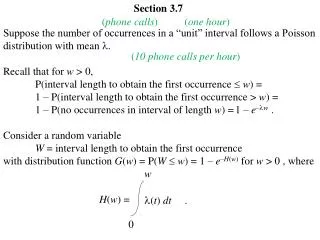
Section 3.7. ( phone calls ). ( one hour ). Suppose the number of occurrences in a “unit” interval follows a Poisson distribution with mean . Recall that for w > 0, P(interval length to obtain the first occurrence w ) =

Section 3.7
E N D
Presentation Transcript
Section 3.7 (phone calls) (one hour) Suppose the number of occurrences in a “unit” interval follows a Poisson distribution with mean . Recall that for w > 0, P(interval length to obtain the first occurrence w) = 1 – P(interval length to obtain the first occurrence > w) = 1 – P(no occurrences in interval of length w) = . Consider a random variable W = interval length to obtain the first occurrence with distribution function G(w) = P(Ww) = 1 – e–H(w) for w > 0 , where H(w) = (10 phone calls per hour) 1 – e–w w (t) dt . 0
If the function (t) is a constant, say , then H(w) = , so that the p.d.f. of W is g(w) = which is the p.d.f. for an distribution. A non-constant function (t) implies that the mean of the Poisson process changes over an interval. For instance, the number of occurrences in a “unit” interval may steadily increase (or decrease). We observe that in general, H/(w) = , so that the p.d.f. of W is g(w) = When W represents length of life (for an item or living organism), (w) is called the failure rate or force of mortality, and we find that (w) = If H(w) = for > 0 and > 0, we say W has a Weibull distribution. w e–w if w > 0 , 1 — exponential( ) (phone calls per hour) (increase as time goes on) (w) H/(w)e–H(w) = (w)e–H(w) if w > 0 . Consider (t) = 10 versus (t) = 5t / 2 when W = hours until first phone call g(w) —— = e–H(w) g(w) ———— . 1 – G(w) w —
For W = hours until first phone call, compare P(W > 1/10) when (t) = 10 and (t) = 5t / 2. 10e–10wif w > 0 . When (t) = 10, the p.d.f. of W is P(W> 1/10) = When (t) = 5t / 2, the p.d.f. of Wis P(W> 1/10) = We can say that W has a Weibull distribution with = and = 1 1/10 e–1 = 0.3679 2 (5w/2)e–(5/4)wif w > 0 . We can say that W has a Weibull distribution with = and = 2 2/5 e–1/80 = 0. 9876
1. A random variable W has p.d.f. g(w) = H/(w)e–H(w)if w > 0 , where H(w) = 243w5/3. Find the values of and so that we may write w — H(w) = in order to demonstrate that W has a Weibull distribution. = = 5/3 1/27
2. (a) Suppose the random variable Wrepresents length of life and has p.d.f. g(w) = H/(w)e–H(w)if w > 0 , with an exponential force of mortality (w) = for a > 0 and b > 0. g(w) ———— = aebw 1 – G(w) Find the distribution function for W. w w aebw– a ——— b H(w) = (t) dt = aebtdt = 0 0 0 if w 0 if 0 < w The distribution function for W is G(w) = a–aebw ——— b 1 – exp
(b) Find the p.d.f. for W (known as Gompertz law). a–aebw ——— b The p.d.f. for W is g(w) = if w > 0 . aebwexp
Let X be a random variable with c.d.f. F(x). In general, for any value v, P(X = v) = P(Xv) P(X < v) = P(Xv) Lim P(Xx) = x v F(v) LimF(x) . x v 0 if x < 5 1/4 if 5 x < 6 (x 5)/4 if 6 x < 9 1 if 9 x Example. Let X be a random variable with c.d.f. F(x) = Suppose v is a value less than 5, say 4.8. P(X= v) = P(X = 4.8) = 0 0 = 0 1 F(4.8) Lim F(x) = x 4.8 3/4 1/2 1/4 0 5 6 7 8 9
0 if x < 5 1/4 if 5 x < 6 (x 5)/4 if 6 x < 9 1 if 9 x Example. Let X be a random variable with c.d.f. F(x) = Suppose v is 5. P(X= v) = P(X = 5) = 1 3/4 1/4 0 = 1/4 F(5) Lim F(x) = x 5 1/2 1/4 0 5 6 7 8 9 Suppose v is a value greater than 5 but less than 6, say 5.8. P(X= v) = P(X = 5.8) = 1/4 1/4 = 0 F(5.8) Lim F(x) = x 5.8
0 if x < 5 1/4 if 5 x < 6 (x 5)/4 if 6 x < 9 1 if 9 x Example. Let X be a random variable with c.d.f. F(x) = Suppose v is a value such that 6 v < 9, say 7.5. P(X= v) = P(X = 7.5) = 1 3/4 F(7.5) Lim F(x) = x 7.5 1/2 5/8 (7.5 5)/4 = 0 1/4 0 5 6 7 8 9 Suppose v is a value greater than or equal to 9, say 9.8. P(X= v) = P(X = 9.8) = 1 1 = 0 F(9.8) Lim F(x) = x 9.8
0 if x < 5 1/4 if 5 x < 6 (x 5)/4 if 6 x < 9 1 if 9 x Example. Let X be a random variable with c.d.f. F(x) = Consequently, we see that if v 5, then P(X= v) = 0 but P(X = 5) = 1 1/4 3/4 1/2 1/4 0 5 6 7 8 9 We also see that P(6 < X 9) = P(X 9) P(X 6) = F(9) F(6) = 1 1/4 = 3/4 We see then that the space of X is {5} {x | 6 < x < 9}
We see then that the space of X is {5} {x | 6 < x < 9} The random variable X is not a discrete type random variable and is not a continuous type random variable; X is called a random variable of the mixed type. What kind of random variable X could have this space? A dart is thrown at a circular board of radius 9 inches. If the dart lands in the area between 3 and 9 inches from the center, a score of 6 is assigned; if the dart lands within 3 inches of the center, then a score of 9 x is assigned where x is the distance from the center. Yellow Area Score = 6 Blue Area Score = 9 x where x = inches from the center.
Let F(x) be the distribution function for a random variable X, then (1) F(x) must be an function, (2) as x –, F(x) , and (3) as x +, F(x) . increasing 0 1 If there exists a discrete set of points at which F(x) is discontinuous with F/(x) = 0 at all other points, then X must be a type random variable whose space is the set of points of discontinuity. (The probability of observing a given value in the space of X is equal to the “length of the jump in F(x)” at the given value.) discrete If F(x) is continuous everywhere, then X is a type random variable whose space is the set of points where F/(x) > 0 (i.e., the set of points where F(x) is strictly increasing). continuous If there exists a discrete set of points at which F(x) is discontinuous and also one or more intervals where F/(x) > 0, then X is called a random variable of the mixed type. Such a random variable is neither of the discrete type or the continuous type and has no p.m.f. or p.d.f. The space of X consists of the union of the set of points of discontinuity and the intervals where F/(x) > 0.
3. (a) For each distribution function, (1) sketch a graph, and (2) either find the corresponding p.m.f. or p.d.f., or state why no p.m.f. or p.d.f. can be found. 1 X1 has distribution function F1(x) = 1 –——— if – <x < . (1 + ex) 1 1/2 0 X1 is a continuous type random variable with p.d.f. f1(x) = F1(x) = ex ——— if – <x < . (1 + ex)2
0 if x<– 3 (x3 + 27) / 35 if – 3x < 2 1 if 2 x (b) X2 has distribution function F2(x) = 1 – 3 0 2 X2 is a continuous type random variable with p.d.f. f2(x) = F2(x) = 3x2 — if – 3x < 2 . 35
0 if x<– 2 1/6 if – 2x < 0 1/3 if 0x < 2 2/3 if 2 x<4 11/12 if 4x < 6 1 if 6 x (c) X3 has distribution function F3(x) = 1 11/12 2/3 1/3 1/6 – 2 0 2 4 6 1/6 if x = – 2 1/6 if x = 0 1/3 if x = 2 1/4 if x = 4 1/12 if x = 6 X3 is a discrete type random variable. The space of X is The p.m.f. of X is f3(x) = {– 2, 0, 2, 4, 6}.
0 if x<– 2 (x + 2) / 12 if – 2x < 0 (2 + 3x ) / 12 if 0x < 4 11 / 12 if 4 x<5 1 if 5 x X4 has distribution function F4(x) = (d) 1 11/12 2/3 1/6 – 2 0 2 4 5 X4 has a distribution of the mixed type. X4 has no p.m.f. or p.d.f. The space of X4 is {x | – 2 < x < 4} {4,5}.
0 if x<– 2 (x + 2) / 12 if – 2x < 0 (5 + 3x ) / 12 if 0x < 4 11 / 12 if 4 x<5 1 if 5 x (e) X5 has distribution function F5(x) = 1 11/12 5/12 1/6 – 2 0 2 4 5 X5 has a distribution of the mixed type. X5 has no p.m.f. or p.d.f. The space of X5 is {x | – 2 < x < 0} {0} {x | 0 < x < 4} {5}.
4. An ordinary, fair, six-sided die is rolled, and each of the two spinners displayed on the right are spun, with the random variables Y1 and Y2 respectively being set equal to the numbers selected from Spinner #1 and Spinner #2. Note that Y1 and Y2 have respective U(2,2) and U(3,5) distributions. The random variable X is defined as follows: Spinner #1 2 1 1 0 Y1 if the die roll results in 1 2 if the die roll results in 2 Y2 if the die roll results in 3, 4, or 5 6 if the die roll results in 6 Spinner #2 3 X = 4.5 3.5 (a) Find the distribution function of X. 4
The space of X is {x | – 2 < x < 2} {2} {x | 3 < x < 5} {6} P(Xx) = F(x) = 0 if x<– 2 In order for –2 < X < 2, the die roll must result in 1, so that X = Y1 . For –2 < x < 2, P(Xx) = P({die roll results in 1} {Y1x}) = (1/6) (2 + x) /4 P(die roll results in 1) P(Y1x) = 2 + x ——— if – 2x< 2 24 P(Xx) = F(x) = In order for X = 2, the die roll must result in 2, and P(X = 2) = We see then that P(Xx) = for 2 x< 3. 1/6 . 1/3
0 if x<– 2 2 + x ——— if – 2x < 2 24 1 — if 2x < 3 3 F(x) = 3x 5 ——— if 3 x < 5 12 In order for 3 <X < 5, the die roll must result in 3, 4, or 5, so that X = Y2 . For 3 <x<5, P(Xx) = P({X< 3} {3 Xx}) = P(X < 3) + P(3 Xx) = 1/3 + P(3 Xx) = 1/3 + P({die roll results in 3, 4, or 5} {Y2x}) = 1/3 + (1/2) (x 3) /2 1/3 + P(die roll results in 3, 4, or 5) P(Y2x) =
It is not possible that 5<X < 6, and in order that X = 6, the die roll must result in 6, and P(X = 6) = We see then that P(Xx) = for 5 x< 6. 0 if x<– 2 2 + x ——— if – 2x < 2 24 1/6 . 5/6 1 — if 2x < 3 3 F(x) = 3x 5 ——— if 3 x < 5 12 5 — if 5x < 6 6 1 if 6 x
(b) Graph the distribution function of X. 0 if x<– 2 2 + x ——— if – 2x < 2 24 1 — if 2x < 3 3 F(x) = 3x 5 ——— if 3 x < 5 12 1 5/6 5 — if 5x < 6 6 1 if 6 x 1/3 1/6 – 2 0 2 4 6
When X is a random variable of the mixed type, the expected value of a function u(X) is calculated by applying the following rules: (1) (2) (3) Multiply each value u(x) corresponding to the discrete list of values for x at which F(x) is discontinuous by its probability (i.e., by the “length of the jump in F(x)” at x). Integrate u(x)F/(x) over each interval where F/(x) > 0. Sum the results obtained from (1) and (2).
(c) Find E(X). 0 if x<– 2 2 + x ——— if – 2x < 2 24 1 — if 2x < 3 3 F(x) = 3x 5 ——— if 3 x < 5 12 5 — if 5x < 6 6 1 (6) — + 6 1 (2) — + 6 E(X) = 2 5 1 if 6 x 0 + 2 = 10 — 3 1 — + 1 + 3 1 x— dx + 24 1 x— dx= 4 –2 3
5. (a) For each random variable, graph the distribution function, and find the expected value. The random variable W = "the length of time in hours a brand W light bulb will burn" has distribution function 0 if w < 0 1 – e–w/300 if 0 w F(w) = F(w) 1 0 Note that W is a continuous type random variable with p.d.f. f(w) = F(w) = e–w/300 —— if 0 <w < 300 (an exponential(300) p.d.f.). E(W) = 300
(b) The random variable X = "the length of time in hours a brand X light bulb will burn" has distribution function 0 if x < 0 1 – (9/10)e–x/300 if 0 x G(x) = G(x) 1 1/10 0 X has a distribution of the mixed type. X has no p.m.f. or p.d.f. 1 (0) — + 10 9e–x/300 x——— dx = 3000 9 e–x/300 — x—— dx = 10 300 9 — (300) = 10 E(X) = 270 0 0
(c) The random variable Y = "the length of time in hours a brand Y light bulb will burn" has distribution function 0 if y < 0 1 – (9/10)e–y/300 if 0 y < 120 1 if 120 y H(y) = H(y) 1 1 – 0.9e–2/5 1/10 0 120 Y has a distribution of the mixed type. Y has no p.m.f. or p.d.f.
120 1 (0) — + 10 3e–y/300 y——— dy + 1000 E(Y) = (120) (0.9e–2/5) = 0 120 – 3(900 + 3y) e–y/300 ———————— + 10 108 e–2/5 = y = 0 – 3(900 + 360) e–2/5 2700 ———————— + —— + 108 e–2/5 = 10 10 270 – 270 e–2/5

