Download
1 / 17
180 likes | 209 Vues
Obtain atmospheric fields for sustainable climatic simulations in following IPCC emission scenarios. Utilize SEB model SURFEX for long-term projections from 2000-2100 based on RCM projections. Methodology involves classification of observational cycles for diverse weather types and cluster reconstructions.

E N D
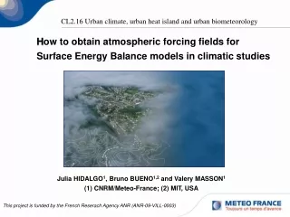
CL2.16 Urban climate, urban heat island and urban biometeorology How to obtain atmospheric forcing fields for Surface Energy Balance models in climatic studies Julia HIDALGO1, Bruno BUENO1,2 and Valery MASSON1(1) CNRM/Meteo-France; (2) MIT, USA This project is funded by the French Reserach Agency ANR (ANR-09-VILL-0003)
Objective: • To provide representative atmospheric fields for a project related with climate change impact in future energy demand in Paris • to be used in long-term off-line simulations (2000-2100) • performed with the SEB model SURFEX (ISBA+TEB) • atmospheric fields are based on existing future projections of climate from Regional Climate Models: ENSEMBLES; MPI; CNRM • for a variety of IPCC emissions scenarios: Nakicenovic et al. (2000)
Key aspects of the study: Related to the temporal frequency of RCM outputs 2. Related to the urban representation in RCMs
Key aspects: Related to the temporal frequency SEB models need: • T; q; U,V; P; PP; +3 radiatif components (Lw, dir_sw, scat_sw) • z = canopy level. Hourly frenquency • Future climate projections currently available for Europe: • T mean,max,min; Hu mean,max,min; U, Vmean; Pmean ; PPmean ; RGmean RAmean • z = 2 m; time-period 1961- 2100 Methodology: - To classify hourly observational diurnal cycles to obtain a collection of clusters that represents the diversity of weather types affecting the site. - To use it to reconstruct the future projections at hourly frequency.
1. Clustering past observations 10years; 1h; ff, dd, T, HU, P, PP 30 years; 3h frequency; ff, dd, T, HU 1961 1990 1998 2008 • Statistic method: K-means • variables included as inputs: Tmax -Tmin, q, ff, dd, pp • Objective: (ΔT(h)mean_season)k 28070001. CHARTRES PARIS Shape: deviation to the mean value
1. Clustering past observations 10years; 1h; ff, dd, T, HU, P, PP 30 years; 3h frequency; ff, dd, T, HU 1961 1990 1998 2008 Wind rose observed for PARIS
T(C) time 1. Clustering past observations: Validation & Reconstruction Specific Humidity Temperature Observations Reconstruction
T(C) time 1. Clustering observations: Validation & Reconstruction Wind force Wind direction Observations Reconstruction
r^2 T ( C ) q (kg/kg) ff (m/s) All points 0,975 0,911 0,701 Mean 1 0,999 0,844 B A Max 0,973 0,978 0,961 Min 0,94 0,917 0,806 C D 1. Clustering observations: Validation & Reconstruction 10years; 1h; ff, dd, T, HU, P, PP 30 years; 3h frequency; ff, dd, T, HU 1961 1990 1998 2008 Standard error r2 1998-2008 Scatter plot: Tall points (A), Tmean (B); Tmax (C) and Tmin (D)
r^2 T ( C ) q (kg/kg) ff (m/s) All points 0,975 0,911 0,701 Mean 1 0,999 0,844 r^2 T ( C ) q (kg/kg) wind Max 0,973 0,978 0,961 All points 0,975 0,911 u Min 0,94 0,917 0,806 Mean 1 1 0,847 Max 0,996 0,873 v Min 0,993 0,987 0,8518 1. Clustering observations: Validation & Reconstruction 10years; 1h; ff, dd, T, HU, P, PP 30 years; 3h frequency; ff, dd, T, HU 1961 1990 1998 2008 • Cluster attribution: AT, AH, (T, Hu)mean, max and min (u-v)mean wind components and PPmean • Reconstruction • Validation 1961-1990: Standard error r2
1. Clustering: Future projections 10years; 1h; ff, dd, T, HU, P, PP 30 years; 3h frequency; ff, dd, T, HU Obs. 1961 1990 1998 2008 It is the degree of fit between the model and the observations. It should be evaluated before future projections analysis. RCM 1961 1990 2100 Bias correction: similar method than in Déqué, M. (2007) Cluster attribution: AT, AH, (T, Hu)mean, max and min (u-v)mean wind components and PPmean 3. Reconstruction 4. Validation 1961-1990
10th, Tmin, winter 10th, Tmin, winter 1. Clustering future projections: exemple ECHAM5-r3_RCA (SMHI center) Standard error r2 • 1961-1990 Control period + Model serie after bias correction * Hourly recontructed model serie
Related to the temporal frequency of RCM outputs 2. Related to the urban representation in RCMs
Key aspects: 2. Related to the urban representation in RCMs RCMs do not use urban parameterizations, so urban climate features are not included in these scenarios.
Key aspects: 2. Related to the urban representation in RCMs RCMs do not use urban parameterizations, so urban climate features are not included in these scenarios. Methodology: To combine UHI scaling laws with the previous hourly regional atmospheric fields to reconstruct the themal spatial structure and day by day evolution.
2. UHI scalings: Night-time: Lu et al. 1997 Day-time: Hidalgo et al. 2008
Thanks for your attention! julia.hidalgo@ymail.com