Differentiation Rules
Differentiation Rules. 3. Rates of Change in the Natural and Social Sciences. 3.8. Rates of Change in the Natural and Social Sciences. We know that if y = f ( x ), then the derivative dy / dx can be interpreted as the rate of change of y with respect to x .

Differentiation Rules
E N D
Presentation Transcript
Rates of Change in the Natural and Social Sciences • We know that if y = f(x), then the derivative dy/dx can be interpreted as the rate of change of y with respect to x. • If x changes from x1to x2, then the change in x is • x = x2 – x1 • and the corresponding change in y is • y = f(x2)– f(x1)
Rates of Change in the Natural and Social Sciences • The difference quotient • is the average rate of change • of y with respect to x over the • interval [x1, x2] and can be • interpreted as the slope of the • secant line PQ in Figure 1. Figure 1 mPQ=average rate of change m = f(x1) = instantaneous rate of change
Rates of Change in the Natural and Social Sciences • Its limit as x 0 is the derivative f(x1), which can therefore be interpreted as the instantaneous rate of change of y with respect to x or the slope of the tangent line at P(x1, f(x1)). • Using Leibniz notation, we write the process in the form
Physics • If s = f(t) is the position function of a particle that is moving in a straight line, then s/t represents the average velocity over a time periodt, and v = ds/dt represents the instantaneousvelocity (the rate of change of displacement with respect to time). • The instantaneousrate of change of velocity with respect to time is acceleration:a(t)=v(t)= s(t). • Nowthat we know the differentiation formulas,we are able to solve problems involving the motion of objects more easily.
Example 1 – Analyzing the Motion of a Particle • The position of a particle is given by the equation • s = f(t) = t3 – 6t2 + 9t • where t is measured in seconds and s in meters. • (a) Find the velocity at time t. • (b) What is the velocity after 2 s? After 4 s? • (c) When is the particle at rest? • (d) When is the particle moving forward (that is, in the positive direction)? • (e) Draw a diagram to represent the motion of the particle. • (f) Find the total distance traveled by the particle during the first five seconds. • (g) Find the acceleration at time t and after 4 s.
Example 1 – Analyzing the Motion of a Particle cont’d • (h) Graph the position, velocity, and acceleration functions for 0 t 5. • When is the particle speeding up? When is it slowing down? • Solution: • (a) The velocity function is the derivative of the position function. • s = f(t) = t3 – 6t2 + 9t • v(t) = = 3t2 – 12t + 9
Example 1 – Solution cont’d • (b) The velocity after 2 s means the instantaneous velocity when t = 2 , that is, • v(2) = • = –3 m/s • The velocity after 4 s is • v(4) = 3(4)2 – 12(4)+ 9 • = 9 m/s = 3(2)2 – 12(2)+ 9
Example 1 – Solution cont’d • (c) The particle is at rest when v(t) = 0, that is, • 3t2 – 12t + 9 = 3(t2 – 4t + 3) • = 3(t – 1)(t – 3) • = 0 • and this is true when t = 1 or t = 3. • Thus the particle is at rest after 1 s and after 3 s.
Example 1 – Solution cont’d • (d) The particle moves in the positive direction when v(t) > 0, • that is, • 3t2 – 12t + 9 = 3(t – 1)(t – 3) > 0 • This inequality is true when both factors are positive • (t > 3) or when both factors are negative (t < 1). • Thus the particle moves in the positive direction in the time intervals t < 1 and t > 3. • It moves backward (in the negative direction) when • 1 < t < 3.
Example 1 – Solution cont’d • (e) Using the information from part (d) we make a schematic sketch in Figure 2 of the motion of the particle back and forth along a line (the s-axis). Figure 2
Example 1 – Solution cont’d • (f) Because of what we learned in parts (d) and (e), we need to calculate the distances traveled during the time intervals [0, 1], [1, 3], and [3, 5] separately. • The distance traveled in the first second is • |f(1) – f(0)| = |4 – 0| • From t = 1 to t = 3 the distance traveled is • |f(3) – f(1)| = |0 – 4| • From t = 3 to t = 5 the distance traveled is • |f(5) – f(3)| = |20 – 0| • The total distance is 4 + 4 + 20 = 28 m. = 4 m = 4 m = 20 m
Example 1 – Solution cont’d • (g) The acceleration is the derivative of the velocity function: • a(t) = • = • = 6t – 12 • a(4) = 6(4) – 12 • = 12 m/s2
Example 1 – Solution cont’d • (h) Figure 3 shows the graphs of s, v, and a. Figure 3
Example 1 – Solution cont’d • (i) The particle speeds up when the velocity is positive and increasing (v and a are both positive) and also when the velocity is negative and decreasing (v and a are both negative). • In other words, the particle speeds up when the velocity and acceleration have the same sign. (The particle is pushed in the same direction it is moving.) • From Figure 3 we see that this happens when 1 < t < 2 and when t > 3.
Example 1 – Solution cont’d • The particle slows down when v and a have opposite signs, that is, when 0 t < 1 and when 2 < t < 3. • Figure 4 summarizes the motion of the particle. Figure 4
Example 2 – Linear Density • If a rod or piece of wire is homogeneous, then its linear • density is uniform and is defined as the mass per unit length • ( = m/l) and measured in kilograms per meter. • Suppose, however, that the rod is not homogeneous but that its mass measured from its left end to a point x is m = f(x), as shown in Figure 5. Figure 5
Example 2 – Linear Density cont’d • The mass of the part of the rod that lies between x = x1 and x = x2 is given by m = f(x2) – f(x1), so the average density of that part of the rod is • If we now let x 0 (that is, x2 x1), we are computing the average density over smaller and smaller intervals. • The linear density atx1 is the limit of these average densities as x 0; that is, the linear density is the rate of change of mass with respect to length.
Example 2 – Linear Density cont’d • Symbolically, • Thus the linear density of the rod is the derivative of mass with respect to length. • For instance, if m = f(x) = where x is measured in meters and m in kilograms, then the average density of the part of the rod given by 1 x 1.2 is • while the density right at x = 1 is
Example 3 – Current is the Derivative of Charge • A current exists whenever electric charges move. Figure 6 shows part of a wire and electrons moving through a plane surface, shaded red. • If Q is the net charge that passes through this surface during a time period t, then the average current during this time interval is defined as Figure 6
Example 3 – Current is the Derivative of Charge cont’d • If we take the limit of this average current over smaller and smaller time intervals, we get what is called the current I at a given time t1: • Thus the current is the rate at which charge flows through a surface. It is measured in units of charge per unit time (often coulombs per second, called amperes).
Example 4 – Rate of Reaction • A chemical reaction results in the formation of one or more substances (called products) from one or more starting materials (called reactants). • For instance, the “equation” • 2H2 + O2 2H2O • indicates that two molecules of hydrogen and one molecule of oxygen form two molecules of water. • Let’s consider the reaction • A + B C • where A and B are the reactants and C is the product.
Example 4 – Rate of Reaction cont’d • The concentration of a reactant A is the number of moles (1 mole = 6.022 1023 molecules) per liter and is denoted by [A]. • The concentration varies during a reaction, so [A], [B], and [C] are all functions of time (t). • The average rate of reaction of the product C over a time interval t1tt2 is
Example 4 – Rate of Reaction cont’d • But chemists are more interested in the instantaneous rate of reaction, which is obtained by taking the limit of the average rate of reaction as the time interval t approaches 0: • rate of reaction • Since the concentration of the product increases as the reaction proceeds, the derivatived[C]/dt will be positive, and so the rate of reaction of C is positive. • The concentrationsof the reactants, however, decrease during the reaction, so, to make the rates of reactionof A and B positive numbers, we put minus signs in front of the derivativesd[A]/dt and d[B]/dt.
Example 4 – Rate of Reaction cont’d • Since [A] and [B] each decrease at the same rate that [C] increases, we have • rate of reaction • More generally, it turns out that for a reaction of the form • aA + bB cC + dD • we have • The rate of reaction can be determined from data and graphical methods. In some cases there are explicit formulas for the concentrations as functions of time, which enable us to compute the rate of reaction.
Example 5 – Compressibility • One of the quantities of interest in thermodynamics is compressibility. If a given substance is kept at a constant temperature, then its volume V depends on its pressure P. We can consider the rate of change of volume with respect to pressure—namely, the derivative dV/dP. As P increases, V decreases, so dV/dP < 0. • The compressibility is defined by introducing a minus sign and dividing this derivative by the volume V:
Example 5 – Compressibility cont’d • Thus βmeasures how fast, per unit volume, the volume of a substance decreases as the pressure on it increases at constant temperature. • For instance, the volume V (in cubic meters) of a sample of air at 25C was found to be related to the pressure P (in kilopascals) by the equation • The rate of change of V with respect to P when P = 50 kPa is
Example 5 – Compressibility cont’d • = –0.00212 m3/kPa • The compressibility at that pressure is • = 0.02 (m3/kPa)/m3
Example 6 – Rate of Growth of a Population • Let n = f(t) be the number of individuals in an animal or plant population at time t. • The change in the population size between the times t = t1 and t = t2 is n = f(t2) – f(t1), and so the average rate of growth during the time period t1tt2 is • average rate of growth • The instantaneous rate of growth is obtained from this average rate of growth by letting the time period t approach 0: • growth rate
Example 6 – Rate of Growth of a Population cont’d • Strictly speaking, this is not quite accurate because the actual graph of a population function n = f(t) would be a step function that is discontinuous whenever a birth or death occurs and therefore not differentiable. • However, for a large animal • or plant population, we can • replace the graph by a smooth • approximating curve as in • Figure 7. Figure 7 A smooth curve approximating a growth function
Example 6 – Rate of Growth of a Population cont’d • To be more specific, consider a population of bacteria in a homogeneous nutrient medium. • Suppose that by sampling the population at certain intervals it is determined that the population doubles every hour. • If the initial population is n0 and the time t is measured in hours, then • f(1) = 2f(0) • f(2) = 2f(1) • f(3) = 2f(2) • In general, • f(t) = 2tn0 = 2n0 = 22n0 = 23n0
Example 6 – Rate of Growth of a Population cont’d • The population function is n0 = n02t. • We have shown that • So the rate of growth of the bacteria population at time t is
Example 6 – Rate of Growth of a Population cont’d • For example, suppose that we start with an initial population of n0 = 100 bacteria. • Then the rate of growth after 4 hours is • This means that, after 4 hours, the bacteria population is growing at a rate of about 1109 bacteria per hour.
Example 7 – Blood Flow • When we consider the flow of blood through a blood vessel,such as a vein or artery, we can model the shape of the blood vessel by a cylindrical tube with radius R and length l as illustrated in Figure 8. • Because of friction at the walls of the tube, the velocity v of the blood is greatest along the central axis of the tube and decreases as the distance r from the axis increases until v becomes 0 at the wall. Figure 8 Blood flow in an artery
Example 7 – Blood Flow cont’d • The relationship between v and r is given by the law oflaminar flow discovered by the French physician Jean-Louis-Marie Poiseuille in 1840. • This law states that • where is the viscosity of the blood and P is the pressure difference between the ends of the tube. • If P and l are constant, then v is a function of r with domain [0, R].
Example 7 – Blood Flow cont’d • The average rate of change of the velocity as we move from r = r1 outward to r = r2 is given by • and if we let r 0, we obtain the velocity gradient, that is, the instantaneous rate of change of velocity with respect to r: • Using Equation 1, we obtain
Example 7 – Blood Flow cont’d • For one of the smaller human arteries we can take = 0.027, R = 0.008 cm, l = 2 cm, and P = 4000 dynes/cm2, which gives • 1.85 104(6.4 10–5 – r2) • At r = 0.02 cm the blood is flowing at a speed of • v(0.002) 1.85 104(64 10–6 – 4 10–6) • = 1.11 cm/s • and the velocity gradient at that point is
Example 7 – Blood Flow cont’d • To get a feeling for what this statement means, let’s change our units from centimeters to micrometers (1 cm = 10,000 m). Then the radius of the artery is 80 m. • The velocity at the central axis is 11,850 m/s, which decreases to 11,110 m/s at a distance of r = 20 m. • The fact that dv/dr = –74 (m/s)/m means that, when r = 20 m, the velocity is decreasing at a rate of about 74 m/s for each micrometer that we proceed away from the center.
Example 8 – Marginal Cost • Suppose C(x) is the total cost that a company incurs in • producing x units of a certain commodity. • The function C is called a cost function. If the number of items produced is increased from x1 to x2, then the additional cost is C = C(x2) – C(x1), and the average rate of change of the cost is
Example 8 – Marginal Cost cont’d • The limit of this quantity as x 0, that is, the instantaneous rate of change of costwith respect to the number of items produced, is called the marginal cost by economists: • marginal cost • [Since xoften takes on only integer values, it may not make literal sense to let x approach 0, but we can always replace • C(x) by a smooth approximating function as inExample 6.] • Taking x = 1 and n large (sothat x is small compared ton), we have • C(n) ≈C(n + 1)–C(n)
Example 8 – Marginal Cost cont’d • Thus the marginal cost of producing n units is approximately equal to the cost of producing one more unit, the (n + 1)st unit. • It is often appropriate to represent a total cost function by a polynomial • C(x) = a + bx + cx2 + dx3 • where a represents the overhead cost (rent, heat, maintenance) and the other terms represent the cost of raw materials, labor, and so on. (The cost of raw materials may be proportional to x, but labor costs might depend partly on higher powers of x because of overtime costs and inefficiencies involved in large-scale operations.)
Example 8 – Marginal Cost cont’d • For instance, suppose a company has estimated that the cost (in dollars) of producing x items is • C(x) = 10,000 + 5x + 0.01x2 • Then the marginal cost function is • C(x) = 5 + 0.02x • The marginal cost at the production level of 500 items is • C(500) = 5 + 0.02(500) • = $15/item
Example 8 – Marginal Cost cont’d • This gives the rate at which costs are increasing with respect to the production level when x = 500 and predicts the cost of the 501st item. • The actual cost of producing the 501st item is • C(501) – C(500) = [10,000 + 5(501) +0.01(501)2] • – [10,000 + 5(500) +0.01(500)2] • = $15.01 • Notice that C(500) ≈ C(501) – C(500).
Other Sciences • Rates of change occur in all the sciences. A geologist is interested in knowing the rate at which an intruded body of molten rock cools by conduction of heat into surrounding rocks. • An engineer wants to know the rate at which water flows into or out of a reservoir. • An urban geographer is interested in the rate of change of the population density in a city as the distance from the city center increases. • A meteorologist is concerned with the rate of change of atmospheric pressure with respect to height.