Understanding Matrices and Row Operations in Linear Systems
This guide explores the fundamentals of matrices and row operations essential for solving linear systems. It defines different types of matrices, including square, coefficient, and augmented matrices. You will learn about elementary row operations such as row interchange, scaling, and addition, which are crucial for transforming matrices into row echelon or reduced row echelon forms. The document provides a step-by-step approach to applying Gaussian elimination to find unique solutions or identify inconsistencies in systems of equations. **Relevant

Understanding Matrices and Row Operations in Linear Systems
E N D
Presentation Transcript
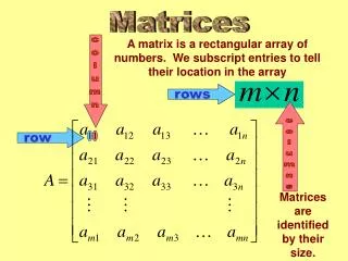
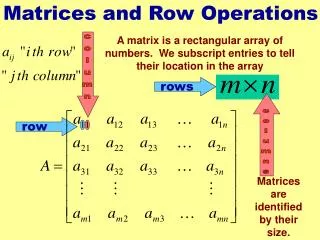
Matrices and Row Operations column rows row columns A matrix is a rectangular array of numbers. We subscript entries to tell their location in the array Matrices are identified by their size.
main diagonal A matrix that has the same number of rows as columns is called a square matrix.
Coefficient matrix If you have a system of equations and just pick off the coefficients and put them in a matrix it is called a coefficient matrix.
Augmented matrix If you take the coefficient matrix and then add a last column with the constants, it is called the augmented matrix. Often the constants are separated with a line.
Elementary Row Operations Operations that can be performed without altering the solution set of a linear system 1. Interchange any two rows 2. Multiply every element in a row by a nonzero constant 3. Add elements of one row to corresponding elements of another row We are going to work with our augmented matrix to get it in a form that will tell us the solutions to the system of equations. The three things above are the only things we can do to the matrix but we can do them together (i.e. we can multiply a row by something and add it to another row).
Row Echelon Form We use elementary row operations to make the matrix look like the one below. The # signs just mean there can be any number here---we don’t care what. "The Goal" After we get the matrix to look like our goal, we put the variables back in and use back substitution to get the solutions.
Use row operations to obtain echelon form: We already have the 1 where we need it. Work on this column first. Get the 1 and then use it as a “tool” to get zeros below it with row operations. The augmented matrix We’ll take row 1 and multiply it by 3 and add to row 2 to get a 0. The notation for this step is 3r1 + r2 we write it by the row we replace in the matrix (see next screen). "The Goal"
3r1 + r2 2r1 + r3 Now our first column is like our goal. 2r1 2 4 2 2 3r1 3 6 3 3 + r3 + r2 2 6 7 1 3 5 1 3 0 2 5 1 0 1 2 0 Now we’ll use 2 times row 1 added to row 3 to get a 0 there.
r2 −2r2 + r3 We need a 1 in the second row second column so we’ll multiply row 2 by −1 We’ll use row 2 with the 1 as a tool to get a 0 below it by multiplying it by −2 and adding to row 3 −2r2 0 −2 −4 0 the second column is like we need it now + r3 0 2 5 −1 0 0 1 −1 Now we’ll move to the second column and do row operations to get it to look like our goal.
z column y column x column equal signs Substitute −1 in for z in second equation to find y Substitute −1 in for z and 2 for y in first equation to find x. Now we’ll move to the third column and we see for our goal we just need a 1 in the third row of the third column. We have it so we’ve achieved the goal and it’s time for back substitution. We put the variables and = signs back in. Solution is: (−2 , 2 , −1)
Solution is: (−2 , 2 , −1) This is the only (x , y , z) that make ALL THREE equations true. Let’s check it. These are all true. Geometrically this means we have three planes that intersect at a point, a unique solution.
Reduced Row Echelon Form To obtain reduced row echelon form, you continue to do more row operations to obtain the goal below. "The Goal" This method requires no back substitution. When you put the variables back in, you have the solutions.
Let’s try this method on the problem we just did. We take the matrix we ended up with when doing row echelon form: −2r2+r1 3r3+r1 −2r3+r2 Let’s get the 0 we need in the second column by using the second row as a tool. Notice when we put the variables and = signs back in we have the solution Now we’ll use row 3 as a tool to work on the third column to get zeros above the 1. "The Goal"
The process of reducing the augmented matrix to echelon form or reduced echelon form, and the process of manipulating the equations to eliminate variables, is called: Gaussian Elimination
Let’s try another one: The augmented matrix: We’ll now use row 1 as our tool to get 0’s below it. r1 −r2 We have the first column like our goal. On the next screen we’ll work on the next column. −2r1+r2 −7r1+r3 If we subtract the second row from the first we’ll get the 1 we need for the first column. "The Goal"
We’ll now use row 2 as our tool to get 0’s below it. Wait! If you put variables and = signs back in the bottom equation is 0 = −19 a false statement! −1/5r2 10r2+r3 INCONSISTENT - NO SOLUTION If we multiply the second row by a −1/5 we’ll get the one we need in the second column. "The Goal"
One more: r1 −r3 1/3r2 −9r2+r3 Oops---last row ended up all zeros. Put variables and = signs back in and get 0 = 0 which is true. This is the dependent case. We’ll figure out solutions on next slide. −2r1+r2 −4r1+r3 "The Goal"
put variables back in solve for x & y Let’s go one step further and get a 0 above the 1 in the second column No restriction on z x yz 3r2+r1 Infinitely many solutions where z is any real number
works in all 3 What this means is that you can choose any real number for z and put it in to get the x and y that go with it and these will solve the equation. You will get as many solutions as there are values of z to put in (infinitely many). The solution can be written: (z + 2 , z + 1 , z) Let’s try z = 1. Then y = 2 and x = 3 Let’s try z = 0. Then y = 1 and x = 2 Infinitely many solutions where z is any real number
Acknowledgement I wish to thank Shawna Haider from Salt Lake Community College, Utah USA for her hard work in creating this PowerPoint. www.slcc.edu Shawna has kindly given permission for this resource to be downloaded from www.mathxtc.com and for it to be modified to suit the Western Australian Mathematics Curriculum. Stephen Corcoran Head of Mathematics St Stephen’s School – Carramar www.ststephens.wa.edu.au