
1. Electrostatics
E N D
Presentation Transcript
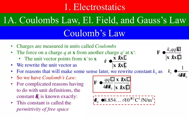
1. Electrostatics 1A. Coulombs Law, El. Field, and Gauss’s Law Coulomb’s Law • Charges are measured in units called Coulombs • The force on a charge q at x from another charge q' at x': • The unit vector points from x' to x • We rewrite the unit vector as • For reasons that will make some sense later, we rewrite constant k1 as • So we have Coulomb’s Law: • For complicated reasons havingto do with unit definitions, theconstant 0 is known exactly: • This constant is called the permittivity of free space
Multiple Charges, and the Electric Field • If there are several charges q'i,you can add the forces: • If you have a continuous distributionof charges (x), you can integrate: • In the modern view, such “action at a distance” seems unnatural • Instead, we claim that there is anelectric field caused by the other charges • Electric field has units N/C or V/m • It is the electric field thatthen causes the forces
Gauss’s Law: Differential Version • Let’s find the divergenceof the electric field: • From four slides ago: • We therefore have: • Gauss’s Law (differential version): • Notice that this equation is local
Gauss’s Law: Integral Version • Integrate this formula overan arbitrary volume • Use the divergence theorem: • q(V) is the charge inside the volume V • Integral of electric field over area is called electric flux Why is it true? • Consider a charge in a region • Electric field from a charge inside a regionproduces electric field lines • All the field lines “escape” the regionsomewhere • Hence the total electric flux escaping must beproportional to amount of charge in the region q
Sample Problem 1.1 (1) A charge q is at the center of a cylinder of radius r and height 2h. Find the electric flux out of all sides of the cylinder, and check that it satisfies Gauss’s Law • Let’s work in cylindrical coordinates • Electric field is: • Do integral over top surface: • By symmetry, theintegral over the bottomsurface is the same h h z r q h r
Sample Problem 1.1 (2) A charge q is at the center of a cylinder of radius r and height 2h. Find the electric flux out of all sides of the cylinder, and check that it satisfies Gauss’s Law h h • Do integral over lateral surface: • Add in the top and bottom surfaces: z r q h r
Using Gauss’s Law in Problems Gauss’s Law can be used to solve three types of problems: • Total electric flux out of an enclosed region • Simply calculate the total charge inside • Electric flux out of one side of a symmetrical region • Must first argue that the flux out of each side is the same • Electric field in a highly symmetrical problem • Must deduce direction and symmetry of electric field from other arguments • Must define a Gaussian Surface to perform the calculation • Generally use boxes, cylinders or spheres
Sample Problem 1.2 A line with uniform charge per unit length passes through the long diagonal of a cube of side a. What is the electric flux out of one face of the cube? • The long diagonal ofthe cube has a length • The charge inside the cube is therefore • The total electric fluxout of the cube is • If we rotate the cube 120 around the axis, the three faces atone end will interchange • So they must all have the same flux around them • If we rotate the line of charge, the three faces at oneend will interchange with the three faces in back • So front and back must be the same • Therefore, all sixfaces have the same flux
Sample Problem 1.3 A sphere of radius R with total charge Q has its charge spread uniformly over its volume. What is the electric field everywhere? • By symmetry, electric field points directly away from the center • By symmetry, electric field depends only on distance from origin Outside the sphere: • Draw a larger sphere of radius r • Charge inside this sphere is q(r) = Q • By Gauss’s Law, Inside the sphere: • Draw a smaller sphere of radius r • Charge inside this sphere is only • By Gauss’s Law, • Final answer:
Sample Problem 1.4 An infinite line of charge has charge per unit length . What is the electric field everywhere? • Which direction does the electric field point? • Surely, it is radially away from the line • What can it depend on? • Only distance from the line • What Gaussian shape should we use? • Cylinder, length L, radius R, centered on the line • Gauss’s law says: • Enclosed charge is L • End caps have zero dot product • Lateral surface is a (rolled up) rectangle length L width 2R • Solve for E:
1B. Electric Potential Curl of the Electric Field • From homework problem 0.1: • Generalize to origin at x': • Consider the curl of the electric field: • Using Stokes’ theorem, we can getan integral version of this equation:
Electric Field: Discontinuity at a Boundary Consider a surface (locally flat) with a surface charge • How does electric field change across the boundary? • Consider a small thin box of area Acrossing the boundary • Since it is small, assume E is constant over top surface and bottom surface • Use Gauss’s Lawon this small box • Charge inside the box is A • Since box is thin, ignore lateral surface • Consider a small loop of length L penetrating the surface • Use the identity • Ends are short, soonly include the lateral part • So the change in E across the boundary is A L – L
The Electric Potential • In general, any function that has curl zero can be written as a gradient • Proven using Stokes’ Theorem • We therefore write: • is the potential (or electrostatic potential) • Unit is volts (V) It isn’t hard to find an expression for : • First note that • Generalize by shifting: • If we write: • Then it follows that:
Working with the Potential Why is potential useful? • It is a scalar quantity – easier to work with • It is useful when thinking about energy • To be dealt with later How can we compute it? • Direct integration of charge density when possible • We can integrate the electric field • It satisfies the Poisson equation: Solving this equation is one of the main goals of the next couple chapters • There is an ambiguity about , because it is an integral of the electric field • Constant of integration is ambiguous • Normally, resolved by demanding () = 0
Sample Problem 1.5 Find the potential and electric field at all points from a line charge with charge per unit length stretching from z = a to z = b along the z-axis. • Easiest to work in cylindrical coordinates: • Find the potential: • Maple: > Phi:= integrate(1/sqrt((zp-z)^2+rho^2),zp=a..b); • To get electric field, use • Maple:> -expand(simplify(diff(Phi,z)));-diff(Phi,rho);
Sample Problem 1.6 A sphere of radius R with total charge Q has its charge spread uniformly over its volume. What is the potential everywhere? • We already found the electric field • It makes sense that potentialdepends only on r • Relation between potential and electric field • Sowehave • Integrate this in the two regions: • We choose () = 0, so • Want potential continuous at r = R, so • Put it together
Conductors • A conductor is any material that has charges in it that can move freely • If an electric field is present inside a conductor, then: • Charges will shift in response • These shifting charges will create electric fields • They will stop only when all electric fields are cancelled • Therefore, (perfect) conductors have E = 0 inside them • Recall that • Hence potential must be constant in a conductor • Consider Gauss’s law for any shape contained within the interior of a conductor • Since there is no electric field, there is no charge in the interior • There can be charge density on the surface of the conductor • Recall the discontinuity in the electric field at the surface • But it vanishes inside • Therefore, the electric field at the surface of a conductor is
Sample Problem 1.7a A neutral solid conducting sphere of radius R has a cubical cavity of side a inside it, with a charge q at its center. What is the electric field outside the sphere? –q q • Consider any Gaussian surface surrounding the cavity • No electric field, so no charge inside • So the charge q must be balanced by charge –q from the conductor on the inside walls of the cavity • But there must be no net charge on the conductor, so charge + q on the outer surface of the conductor • This surface charge feels no force from the other charges, so it will distribute itself uniformly over the surface • This creates the same field as a point source at x = 0 • Nothing to do with where the charge is • Nothing to do with shape/size, etc. of cavity +q
Sample Problem 1.7b q A neutral solid conducting sphere of radius R has a cubical cavity of side a inside it, with a charge q outside. What is the electric field inside the cavity? • The conductor is at constant potential, = 0. • The potential on the interior surface of the cavity is • There is no charge inside the cavity, so in the cavity, • As we will demonstrate shortly, the value on the boundary plus thevalue of the Laplacian is sufficient to determine the potential • I’m so good, I can get this solution by guess and check: • Check it yourself • Therefore, the electric field inside is • This has nothing to do with the shape of the cavity, the position of q, etc.
Potential and Potential Energy • Consider the formula: • Consider the relationship between energy and potential energy • By comparison, we see that • For example, for two charges q1 and q2 at x1 and x2: • If you have a lot of charges, • The i < j to avoid double counting • This is equivalent to • If you have a continuum of charges, this can be written as • Recall • We therefore have:
Sample Problem 1.7 A sphere of radius R with total charge Q is being approached by a charge q and mass m with speed v from infinity. How fast must q be moving to make it to the center of the sphere? R Q • Use conservation of energy • We already knowthe potential • At infinity, the energy is • At the origin, the charge stops, so • Equating these, we have v q
1C. Boundary Value Problems Definition of the Problem • Sometimes, we don’t know, don’t care, or don’t want todo the work of figuring out the potential everywhere • Sometimes, just want potential in a volume V • Which may be infinite • Poisson equation alone is not sufficient alone to determine potential • You need additional information about what happens to the potential at boundary • This information can take one of two types: • On Dirichletboundary D, the potential is specified • Assume this happens somewhere perhaps x = • On Neumann boundary N, the normal derivative • Goal: find solution to these equations SN SD /n
Uniqueness of Solution? • Could there be two solutions that satisfy all three equations? • If 1 and 2 are both solutions of these, then define: • It follows that • Consider the integral: • Also, do the integral by divergence theorem • On each surface, one of the factors vanishes • The integrand is never negative • Therefore, the only way to make it vanish is for the integrand to vanish • Therefore U is constant • If anywhere we have Dirichlet boundary conditions, then SN SD /n
Finding a “Simple” Solution • Consider the problem witha simple point source at x: • Let’s also let all theboundaryconditions vanish: • We know the solution is unique: • If we had no boundaries, (except at ), solution would be • Let’s call the general solution (with zero boundaries): • These are called Green functions • This solution will have the properties: SN SD /n
How to Find or Check a Green’s Function • Green functionsgenerally look like • The first term satisfies: • It follows that • The F term is just there to make the boundary conditions work out right • It is nonetheless usually hard to find If we think we have G, how do we check it? • Check that the Laplacian satisfies its equation • Check boundary conditions on Dirichlet boundaries (including G(x,) = 0) • Check boundary conditions on any Neumann boundaries SN SD /n
Sample Problem 1.8 Consider the half-space z > 0 with Dirichlet boundary conditions. Show that the function below is the correct Green’s function SD • Since x' = 0 is included in the space, we should have: • We also have the boundary z' = 0, at which we should have: • Finally, we have to check: • We are only interested in points within the allowed region • That means bothz > 0 and z' > 0 • The second delta function can never vanish, so
Using the Green’s Function • G is the problem for a single point source • For a more general source, you would think you could then add the charges to get the general solution, so long as boundary conditions are still zero • Surprisingly, you can use G to get the general solution even when the boundary conditions aren’t zero • We will now demonstrate this SN SD /n
Potential from Green’s Functions (1) • Consider any two functions f and g of x • Consider thefollowing identity: • Swap f and g: • Subtract them: • Integrate usingdivergence theorem: • Turn it around: • Normal derivatives: • Now, change variable x to x',let fbe (x'),and let gbe G(x,x'):
Potential from Green’s Functions (2) • Use the Laplaciansabove on left side: • Do the first integral • Break surface integral into Dirichlet part and Neumann part: SN SD /n
Sample Problem 1.9 (1) Consider the half-space z > 0 conditions. Find the potential everywhere if there is no charge, and its boundary value is as given by • Since we are given potential, we need Dirichlet Green function: • The general solution (dropping the Neumann term): • The normal derivative is out of the region, so • We find: • No charge so SD
Sample Problem 1.9 (2) Consider the half-space z > 0 conditions. Find the potential everywhere if there is no charge, and its boundary value is as given by SD • Can complete the integral by hand using a trig substitution: • Substituting in, we have
1D. Capacitance and Energy Capacitance • Suppose you have conductors (and nothing else) in free space • Potential is constant on each • For each i, set Vi = 1 and Vj = 0 for j i, thenthere is some unique solution to this equation (x): • For arbitrary Vi the solution will be: • The charge on any conductor is then • Define the capacitance: • Units are Farads (F) • Then we see that • Can argue: S1 V1 V2 S2
Sample Problem 1.10 What’s the capacitance of the Earth? • We have only one object, so we write • Treat the Earth as a spherical conductor of radius R = 6370 km • If we place a charge Q on it, the charge distributes itself uniformly over the surface • Electric field will be radially outward and depend only on r • By Gauss’s law, electric field will look like from a point charge: • The potential outside will alsolook like a point charge: • By continuity, the potentialon the surface is then just • Solve for thecapacitance: • Substitute numbers in:
Energy of a System of Conductors V1 • Consider the formula for energy: • Only charge is on the surfaces, so • We therefore have: V2
Another Formula for Energy • Previous formula for potential energy: • Recall: • So we have: • Now use the identity: • We therefore have: • On first term, use divergence theorem • On second term, use E(x) = –(x) • At infinity, E and both vanish • We therefore have • Also equivalent to • Think of this expression as energy density: • Modern viewpoint: The energy density is in the electric field
1E. Variational Method Minimization of Energy • Consider a problem with Dirichlet boundaries • We have an intuitive sense thatsystems try to minimize their energy • Can we find by minimizing this expression? • Not exactly, because we have to make sure is large when is large • For any function (x),consider the functional • We will pick so it hascorrect boundary conditions • We will demonstrate that if we pick = , we minimize this expression SD
Minimizes the Functional • Suppose that and differ by f(x): • Note that f vanishes on the boundary • Then we have • The last term is always positive • So this functional is minimized for the choice = • If we are close (f is small), we will get close (order f2) SD
The Variational Method • Rather than picking a single function, pick a lot with the right boundary conditions • For each of them, find the functional: • Minimize it with respect to all the parameters • Then the approximation for the potential is SD
The Variational Method and Capacitance V • Suppose we have a capacitor with voltage V • Set V = 1 and try to find the potential • Use the variational approach • Minimize • The energy for a capacitor is • The energy is also given by • We therefore have • This is always an overestimate
Sample Problem 1.11 Estimate the capacitance for a cube of side 2a • Place the cube at the origin • Guess the functional form for potential • Must be 1 on the surface • Want it to fall off as 1/r at infinity • By symmetry, assume |x| is largest and x > 0 • Multiply by 6 to account for all the regions • We therefore have • Minimize with respect to the parameter b • Substitute back in
1F. Relaxation Method Potential Can Be Found from Nearby Points • Consider the potential near a point x withno charge density and Dirichlet boundaries • Let’s work in 2D (not sure why) • For a point offset in x-direction or y-direction will be approximately • Add these four points • Wethereforehave
Using a Grid • Set up a rectangular grid: • Label points by i and j • Potential on boundaries is fixed • In the interior, calculate using • Repeat until it converges • Comparably, you can use • Can show a more accurate method would be
Sample Problem 12 A square of side a has potential 0 on three sides and poten-tial 1 on y = a. What is the potential at (x,y) = (a/4 , a/4) • Let’s set up a grid of size a/4 • Need 55 size grid • Set it up in an appropriate program • I used Excel • Type in all the boundary values • Put in one of the formulas • Recalculate repeatedly (F9)until it converges • Increase grid size if you want