Quantitative Inheritance - Pt.1

1. Quantitative Inheritance - Pt.1 Chapter 8

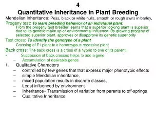
2. Quantitative phenotypes • Continuously variable, expressed as a quantity: • height, weight, running speed, morphology (beak depth, beak width), number of offspring (fitness), IQ score, behavior (novelty seeking), serum cholesterol, etc., etc. • Generally show a bell-shaped (normal) distribution • Are controlled by several to many genes • Are influenced, often strongly, by environment • A main goal of many quantitative genetic studies is to determine the heritability of a trait – the degree to which phenotypic variation among individuals is due to genetic differences among individuals, or the degree to which offspring resemble their parents

3. Quantitative vs. discrete (Mendelian) phenotypes • A “classic” Mendelian phenotype is a trait that is controlled by a single gene and which comes in two discrete “flavors” – dominant and recessive – or three “flavors” if there is co-dominance or incomplete dominance • Classic Mendelian traits show clear-cut phenotypic ratios in controlled crosses, such as the 3:1 F2 ratio in a monohybrid cross with dominance • Because they show continuous, rather than discrete, variation, quantitative phenotypes do not yield clear-cut phenotypic ratios in controlled crosses

4. Some quantitative traits in humans (Fig. 8.1)

5. A short history of quantitative genetics – 1 • Francis Galton (a cousin of Charles Darwin) is the father of quantitative genetics, often referred to in early years as biometrics • Hereditary Genius, 1869 • Note that quantitative genetics developed initially in the absence of any knowledge of Mendelian genetics – based on statistical descriptions of phenotypic correlations between relatives • After the re-discovery of Mendel in 1900, there ensued a long controversy about whether the mechanism of inheritance of quantitative traits was fundamentally different from that of Mendelian traits, and even whether natural selection could act effectively on quantitative traits

6. A short history of quantitative genetics – 2 • Work by Edward East (1916) on inheritance of corolla height in longflower tobacco, and theoretical work by R.A. Fisher reconciled the Mendelians and the biometricians by showing that quantitative inheritance could be explained on the assumption of Mendelian genetics, and with the additional assumptions that several to many genes controlled the variation in the quantitative phenotype and that the phenotype was also affected by environment. • Fisher, R.A. 1918. The correlation between relatives on the supposition of Mendelian inheritance. • This is the paper in which Fisher coined the term “variance” • This is not the only instance that we will see of the close association between quantitative genetics and statistics

7. Inheritance of corolla height in longflower tobacco under the assumption of a single controlling gene and incomplete dominance (Fig. 8.2a)

8. Inheritance of corolla height in longflower tobacco under the assumption of two controlling, independently assorting, incompletely dominant genes, with equal and additive effects on the phenotype (Fig. 8.2b)

9. Inheritance of corolla height in longflower tobacco under the assumption of six controlling, independently assorting, incompletely dominant genes, with equal and additive effects on the phenotype (Fig. 8.2c)

10. Analysis of the 6-locus model • In the 6-locus model on the previous slide, we are not likely to recover the parental phenotypes unless we look at a very large number of F2 individuals • P(homozygous for all lower-case alleles) = (1/4)6 = 1/4096 • This looks like blending inheritance in which the extreme parental phenotypes are not recovered in the F2 • But, according to Mendelian genetics, the parental alleles are still intact

11. Analysis of the 6-locus model(continued) • East realized that, consistent with Mendelian inheritance, most F2 individuals would be heterozygous at most loci and would have intermediate phenotypes • But, he also reasoned that if the parental alleles were still intact, as predicted by Mendelian genetics, he could recover the parental phenotypes by selecting for increased and decreased corolla height starting with the F2

12. Selection on corolla length in longflower tobacco is consistent with Mendelian inheritance (Fig. 8.3)

13. Analysis of selection on corolla height • East was able, with only 3 generations of artificial selection, to recover phenotypes that resembled the parents — the parental alleles were still there — short and tall corollas had not been lost by blending inheritance • In modern terminology, we would say that selection increased the frequencies of alleles that produced the selected phenotype, and more individuals became homozygous for those alleles at more loci • Note that the individuals in each parental strain don’t all have exactly the same phenotype: their variation reflects environmental effects on the phenotype (assuming that they are highly inbred and homozygous)

14. Identifying genes that control variation in quantitative traits — quantitative trait loci (QTLs) • QTL mapping • Candidate loci • Both approaches depend upon the development of molecular genetic technology, particularly DNA sequencing, during the last 10 - 15 years

15. QTL Mapping • Life span in Drosophila melanogaster

16. M1 M2 M3 M4 M5 M6 M7 QTL QTL A hypothetical map of 2 QTLs and 7 markers on a chromosome The Mi are the marker loci. Microsatellite loci are often used as markers. Marker genotype is determined by electrophoresis. Two QTLs are represented by red triangles. Note: we do not know in advance if any QTL are on the chromosome, or, if there are, where they are located

17. M1 M1 QS QS M2 M2 m1 QL m2 c1 c2 c1 c2 m1 QL m2 M1 QS M2 c1 c2 m1 QL m2 Interval Mapping – QTL in interval (1) Short-lived inbred line, S Long-lived inbred line, L P: F1:

18. Interval Mapping – QTL in interval (2) • In the F2, differences in life span among marker genotypes indicate a life span QTL in the marker interval • In the F2, the life span phenotypes of individuals that carry chromosomes with crossovers between the markers give information about where in the interval the QTL is located

19. Interval Mapping – QTL in interval (3) F2 marker genotypeLikely F2 QTL Likely F2 genotype phenotype “Non-crossovers” M1M2/M1M2 QS / QS short life M1M2/m1m2 QS / QL ? m1m2/m1m2 QL / QL long life QTL close to M1QTL close to M2 Crossovers M1m2/M1M2 QS/ QS QL / QS M1m2/m1m2 QS /QL QL / QL m1M2/M1M2 QL / QS QS / QS m1M2/m1m2 QL / QL QS / QL

20. M3 M3 M4 M4 m3 m4 m3 m4 M3 M4 m3 m4 Interval Mapping – no QTL in interval (1) Short-lived inbred line, S Long-lived inbred line, L P: F1:

21. Interval Mapping – no QTL in interval (2) • In the F2, we expect no differences in life span among marker genotypes because there is no QTL in the marker interval

22. Interval Mapping – no QTL in interval (3) F2 marker genotypeLikely F2 QTL Likely F2 genotype phenotype “Non-crossovers” M3M4/M3M4 null average M3M4/m3m4 null average m3m4/m3m4 null average Crossovers M3m4/M3M4 null average M3m4/m3m4 null average m3M4/M3M4 null average m3M4/m3m4 null average

23. QTL Mapping – the Likelihood map • The statistical test of whether or not a QTL is located at a given position on a chromosome is based on a comparison of the likelihood (= probability) of the observed data on the assumption of no QTL at the position versus the likelihood of the data on the assumption that there is a QTL at the position • This allows us to calculate a likelihood ratio (LR) for a QTL at each position along a chromosome, which results in a likelihood map • Peaks in the likelihood map that are above an established threshold for statistical significance indicate the presence and location of a QTL

24. D. melanogaster chromosome 3 likelihood map for life span QTL Each line represents a cross between a different pair of parental lines (horizontal line is the experiment-wise significance threshold, a = 0.05, and the diamonds show marker locations). Red arrows indicate QTL that are present in more than one cross. There is evidence here for at least 4 life span QTL. Forbes, S. N., R. K. Valenzuela, P. Keim, and P. M. Service. 2004. Quantitative trait loci affecting life span in replicated populations of Drosophila melanogaster. I. Composite interval mapping. Genetics 168:301-311.

25. D. melanogaster chromosome 2 likelihood map for life span QTL Each line represents a cross between a different pair of parental lines (horizontal line is the experiment-wise significance threshold, a = 0.05, and the diamonds show marker locations). Red arrows indicate QTL that are present in more than one cross. There is evidence here for at least 1 life span QTL. Forbes, S. N., R. K. Valenzuela, P. Keim, and P. M. Service. 2004. Quantitative trait loci affecting life span in replicated populations of Drosophila melanogaster. I. Composite interval mapping. Genetics 168:301-311.

26. The shortcomings of QTL mapping • Interval mapping is not very precise. Typically it locates QTLs to fairly broad regions of chromosomes. These regions may contain hundreds of genes. • More precision is possible, but with a lot more work, and we are still not likely to identify the actual genes

27. Candidate Loci • Another approach to identifying QTLs is to look directly at genes that are suspected, usually on the basis of known function of the gene product, to play a role in determining a quantitative phenotype • These genes are referred to as candidate genes

28. Analysis of a candidate locus – 1 • Benjamin et al. (1996) looked for a relationship between allelic variation in the gene D4 dopamine receptor (D4DR) and novelty seeking behavior in humans, a quantitative trait as measured by a score on a questionnaire • Dopamine is a neurotransmitter involved in communication between brain cells

29. Analysis of a candidate locus – 2 • Alleles of the D4DR gene vary in the number of copies of a 48 bp tandem repeat (2 - 8 repeats) • Alleles were classified as “short” or “long” • “Novelty seeking” expresses a continuum between “excitable, impulsive, exploratory” personality and “reflective, stoic, rigid” personality

30. Association between genotypes at the D4 dopamine receptor (D4DR) gene and “novelty-seeking score” (Fig 8.10)

31. Analysis of a candidate locus – 3 • Individuals with at least one “long” allele scored, on average, 3 points higher on the questionnaire than did “short” homozygotes • The D4DR gene explains about 3-4% of the variation in novelty seeking scores • That’s not very much. If novelty seeking has reasonably high heritability, we expect that there are other genes that affect it.

32. Measuring heritable variation • How much of the phenotypic variation in a trait is due to genetic differences among individuals? • How much of it is due to environmental effects on individuals? • What is the heritability of a trait?

33. Components of variance • The total variation in a trait is called the phenotypic variance, VP • The variation among individuals that is due to genetic differences among individuals is the genetic variance, VG • The variation among individuals that is due to environmental effects is environmental variance, VE • With some simplifying instructions, VP = VG + VE

34. Broad-sense heritability, H2 • H2 = VG / VP = VG / (VG + VE) • Note: if a population consists of a single clone, all individuals have the same genotype, and VG = 0, so H2 = 0 • On the other hand, if individuals have different genotypes, but environment has no effect on the trait, then VE = 0, and H2 = 1 • The theoretical range of heritability is 0 to 1

35. Additive and dominance genetic variance • The genetic variance can be further decomposed into additive genetic variance, VA, and dominance variance, VD • VG = VA + VD • The additive genetic variance is the part of the phenotypic variation that results from the average effects of alleles when combined at random with other alleles in the population. • The dominance variance is the part of the phenotypic variation that results from the dominance interaction between a pair of alleles at a locus.

36. Additive variance and narrow-sense heritability, h2 • Additive variance is important in sexually reproducing organisms because parents pass on only 1 allele of each gene to offspring — not both alleles • This means that they do not pass on the part of their phenotype that is due to dominance • h2 = VA / VP = VA / (VA + VD + VE) • h2 ≤H2

37. Estimating heritability • The every day sense of heritability is that it describes resemblance between relatives. If a trait is highly heritable, we expect children to strongly resemble their parents • In fact, resemblance between parents and offspring is one way of estimating heritability • In offspring - midparent regression, the slope of the regression line is an estimate of h2

38. Estimating heritability by offspring-parent regression (Fig. 8.11a-c) Heritabilit approximately 0 Midoffspring height (average height of offspring) Midparent height (average height of mother and father Midparent height (average height of mother and father